The Logic of Science

The genetic fallacy: When is it okay to criticize a source?

Posted on January 18, 2016 by Fallacy Man

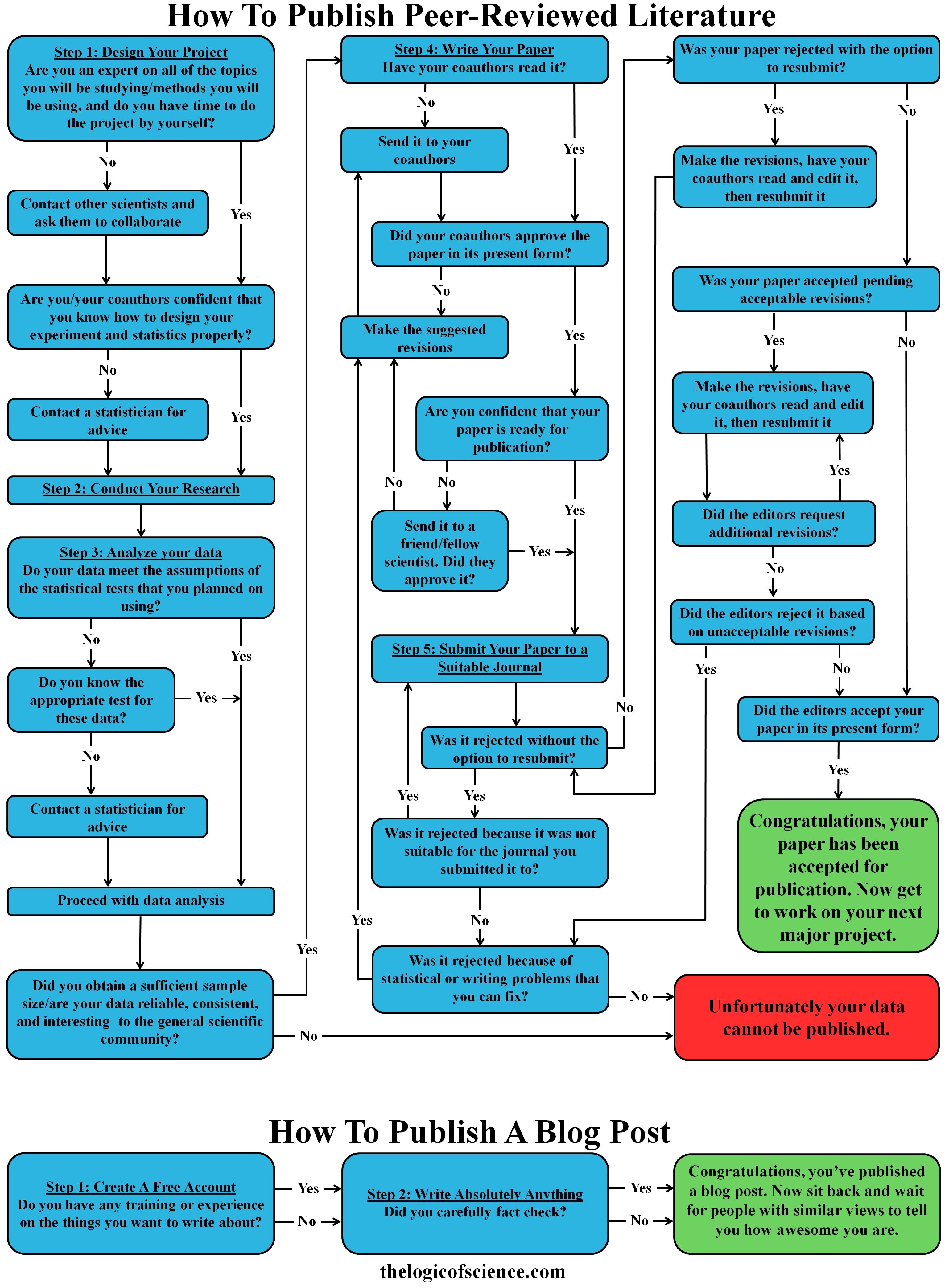
Last week, I wrote a post on the hierarchy of scientific evidence which included the figure to the right. In that post, I explained why some types of scientific papers produced more robust results than others. Some people, however, took issue with that and accused me of committing a genetic fallacy because I was attacking the source of their information rather than the information itself. They were specifically unhappy about my claim that personal anecdotes, gut feelings, counter-factual websites, etc. did not constitute scientific evidence. After all, how dare I assert that their opinions weren’t as valuable as a carefully controlled study (note the immense sarcasm). In reality, of course, my argument was not fallacious, and they were simply misunderstanding how the genetic fallacy works. This misunderstanding is, however, quite common and somewhat understandable. The genetic fallacy can admittedly be very confusing. Therefore, I want to briefly explain what this fallacy is, how to spot it, and when it is and is not acceptable to criticize the source of an argument/piece of information.

If you’re a regular reader of this blog, then much of this may sound very familiar. That is because I have already covered a lot of the key points in a previous post on ad hominem fallacies. The ad hominem fallacy is generally considered to be a type of genetic fallacy; therefore, the same general rules apply.

Note: in this post, I am going to specifically deal with this fallacy as it pertains to scientific issues.

What is the genetic fallacy?
As it’s name suggests, the genetic fallacy results from attacking the source or origin of information, rather than the information itself. If you think about that for a second, the reason for the confusion becomes clear. On the one hand, the reason that genetic fallacies don’t work is obvious: the truth of a claim is not dependent on the one who is making the claim. Even someone who is wrong 99.9% of the time will occasionally be right. On the other hand, however, the source of the information is clearly important. It’s intuitively obvious that not all sources are equal, and some sources are more authoritative than others. Imagine, for example, that during a trial, the prosecution brought in some random guy off of the street and asked him to testify about the forensic evidence of the case. The defense would very correctly attack the source of that information by arguing that this person was not a credentialed expert and, therefore, his testimony should not be trusted. There is obviously nothing fallacious about that, and the prosecution clearly couldn’t respond by accusing the defense of a genetic fallacy (they also couldn’t respond by saying “well he watched some Youtube videos on crime scene investigations and he’s read some blogs and done thousands of hours of research”).

So how do we resolve this apparent dilemma? The answer is that attacking the source of a claim is only fallacious if the source is irrelevant to veracity and trustworthiness of that claim. The Internet Encyclopedia of Philosophy defines it like this (my emphasis):

A critic uses the Genetic Fallacy if the critic attempts to discredit or support a claim or an argument because of its origin (genesis) when such an appeal to origins is irrelevant.

In other words, there is nothing wrong with attacking a source, if the source of the information is actually germane to whether or not you should trust the information. So, if someone cites questionable sources like Youtube videos or personal anecdotes, there is nothing wrong with you saying that we shouldn’t trust that information, because the sources actually are unreliable. That’s no different from not trusting some random guy off the street as an expert witness in a courtroom. Remember, that the burden of proof is always on the person making the claim, so it is their responsibility to provide you with evidence from a trustworthy source. As a result, if they make a claim like, “vaccines are dangerous” and their “evidence” is an Info Wars article, you are under no obligation to discredit that article. Rather, it is their obligation to provide you with evidence from a reliable source.

It’s important to note, however, that you can only use attacks against a source to show that the information cannot be trusted. You cannot use them to say that the information is false. For example, if someone presents you with “evidence” from a Natural News article, there is nothing wrong with saying, “Natural News is not a reliable source, therefore we should not trust that information.” It would, however, be fallacious to say, “Natural News is not a reliable source, therefore that information is wrong” (technically that would be a special case of the fallacy fallacy). Even an extremely unreliable source may be right every once in a while.

In addition to assaults on the source of the information, the genetic fallacy can also occur when you attack the reason for a person holding a particular view. For example, I frequently see creationists attack their opponents by saying, “you only accept evolution because you are an atheist who doesn’t want to believe in God.” Even if that premise was true (which it often isn’t), it’s irrelevant. It has no bearing on whether or not evolution is true, and is, therefore, a genetic fallacy.

Finally, it’s important to realize that for an argument to be a genetic fallacy the assault on the source has to actually be the argument. For example, if you show me a scientific study, and I respond by saying, “well the authors of that study are just ugly idiots so I don’t need to listen to them,” then I would have committed a genetic fallacy (specifically, an ad hominem fallacy). If, however, I explained at length why the study was flawed, then concluded with a Trump-like jab at the authors appearance/intelligence, I would not have committed a fallacy. It would be uncouth and inappropriate for me to do that, but it wouldn’t actually be a fallacy because the attack on the source was tangential to my argument.

Addendum (19-Jan-16): The genetic fallacy also occurs if you assert that something is true because of its source (i.e., the appeal to authority fallacy is actually a type of genetic fallacy), but in this post, my focus was on attacking sources, rather than using them as proof of a position.

The genetic fallacy vs. the hierarchy of scientific evidence
Now that you understand what this fallacy is, let’s bring it to bear on the topic that inspired this post: the hierarchy of scientific evidence. It should by now be clear that using the hierarchy of evidence to assess the validity of a scientific claim is not the same thing as committing a genetic fallacy. Nevertheless, let’s look closer.

First, let’s look at my assertion that personal opinions, anecdotes, anti-science websites, etc. do not count as scientific evidence. It’s worth noting, that I didn’t actually say that they aren’t trustworthy. Rather, I simply said that they aren’t scientific evidence, and that claim is demonstrably true because those sources do not produce evidence via the standards and methodologies of science. Therefore, they are, by definition, not scientific evidence. If I ask someone to give me scientific evidence for a position, then I am asking for actual original research. I want to see the peer-reviewed paper that found the result that they are reporting, not the Youtube video they watched.

flowchart diagram how to publish scientific peer-reviewed paper blog

This flowchart summarizes the steps required to publish a peer-reviewed paper and the steps required to publish a blog post. Take a careful look at this difference, then honestly tell me that you think that blogs are a better source of information about science (more details here).

Nevertheless, although I didn’t claim that non-scientific sources are untrustworthy in the original post, I clearly think that they are. People often take issue with this, but if you stop and think about it for a second, the claim is self-evident. All that I am saying is that for scientific topics, we have to use scientific evidence, which necessarily comes from the peer-reviewed literature. Websites, Youtube videos, etc. are inherently second hand information, which may or may not be reliable. The scientific literature, on the other hand, is primary information. When you read a scientific paper, you can see the actual results of an experiment rather than simply reading someone’s biased explanation of those results. Further, to publish a peer-reviewed paper takes a tremendous amount of work. You have to pass a rigorous peer-review process during which numerous other scientists will evaluate your work to ensure that it was done correctly. In contrast, any idiot with a computer and internet connection can make a website/Youtube video with absolutely no assurance of quality control. To be clear, that doesn’t automatically mean that the information contained in second-hand sources is wrong, but it does mean that you don’t have any reason to trust that information, which is why they aren’t valid sources for scientific topics. Further, websites like Natural News, Info Wars, Answers in Genesis, etc. are notorious for containing inaccurate information, which gives you an extremely strong, relevant, and legitimate reason not to trust them.

Even within the scientific literature, however, you should be looking critically at the sources. Some experimental designs are simply more powerful than others and produce more reliable results. For example, if you have a meta-analysis of randomized controlled trials vs. a cross sectional analysis, it would not be a genetic fallacy to say that the cross sectional analysis is less reliable than the meta-analysis. From a strictly mathematical point of view, cross sectional studies are weak. They simply cannot make causal conclusions. In contrast, randomized controlled trials are very powerful and can make causal conclusions, and meta-analyses are even better because they combine multiple data sets, thus greatly increasing the sample size and reducing the chance of reaching a faulty conclusion. It’s a simple mathematical fact that meta-analyses are better than cross sectional analyses. Therefore, the type of study (i.e., the source of the information) is extremely relevant to the trustworthiness of a study, and using that information in a debate does not constitute a genetic fallacy.

ad hominem fallacy logical fallacy flow chart

Note: this flowchart only works when you are making an attack. Appeals to authority are also a type of genetic fallacy which I did not cover in this post or flowchart (you can find an explanation of them here).

Conclusion
Genetic fallacies occur when you make an irrelevant attack on the source of information rather than the information itself. That does not mean, however, that it is always fallacious to attack the source of information. Some sources clearly are better than others, and the burden of proof is always on the person making the claim. Thus, it is their responsibility to provide high quality sources, and you are not responsible for disproving the information from extremely low quality sources. Nevertheless, determining when attacks on sources are fallacious can admittedly be confusing. Therefore, I have constructed the flowchart on the right to help you determine when you can and cannot attack a source.

Note: Just to be clear, arbitrarily accusing someone of being a shill without providing actual evidence that they are being paid off does not constitute a legitimate, relevant concern.

More posts on logical fallacies:

Posted in Rules of Logic | Tagged ad hominem fallacies, evaluating evidence, logical fallacies, rules of logic | 17 Comments

The hierarchy of evidence: Is the study’s design robust?

Posted on January 12, 2016 by Fallacy Man

People are extraordinarily prone to confirmation biases. We have a strong tendency to latch onto anything that supports our position and blindly ignore anything that doesn’t. This is especially true when it comes to scientific topics. People love to think that science is on their side, and they often use scientific papers to bolster their position. Citing scientific literature can, of course, be a very good thing. In fact, I frequently insist that we have to rely on the peer-reviewed literature for scientific matters. The problem is that not all scientific papers are of a high quality. Shoddy research does sometimes get published, and we’ve reached a point in history where there is so much research being published that if you look hard enough, you can find at least one paper in support of almost any position that you can imagine. Therefore, we must always be cautious about eagerly accepting papers that agree with our preconceptions, and we should always carefully examine publications. I have previously dealt with this topic by describing both good and bad criteria for rejecting a paper; however, both of those posts were concerned primarily with telling whether or not the study itself was done correctly, and the situation is substantially more complicated than that. You see, there are many different types of scientific studies and some designs are more robust and powerful than others. Thus, you can have two studies that were both done correctly, but both reached very different conclusions. Therefore, when examining a paper, it is critical that you take a look at the type of experimental design that was used and consider whether or not it is robust. To aid you in that endeavor, I am going to provide you with a brief description of some of the more common designs, starting with the least powerful and moving to the most authoritative.

Note: Before I begin, I want to make a few clarifications. First, this hierarchy of evidence is a general guideline, not an absolute rule. There certainly are cases where a study that used a relatively weak design can trump a study that used a more robust design (I’ll discuss some of these instances in the post), and there is no one universally agreed upon hierarchy, but it is widely agreed that the order presented here does rank the study designs themselves in order of robustness (many of the different hierarchies include criteria that I am not discussing because I am focusing entirely on the design of the study). Second, the exact order of the designs that I have ranked as “very weak” and “weak” is debatable, but the key point is that they are always considered to be the lowest forms of evidence. Third, for sake of brevity, I am only going to describe the different types of research designs in their most general terms. There are subcategories for most of them which I won’t go into. Fourth, this hierarchy is most germane to issues of human health (i.e., the causes a particular disease, the safety of a pharmaceutical or food item, the effectiveness of a medication, etc.). Many other disciplines do, however, use similar methodologies and much of this post applies to them as well (for example, meta-analysis and systematic reviews are always at the top). Finally, realize that for the sake of this post, I am assuming that all of the studies themselves were done correctly and used the controls, randomization, etc. that are appropriate for that particular type of study. In reality, those are things which you must carefully examine when reading a paper.

Opinions/letters (strength = very weak)
Some journals publish opinion pieces and letters. These are rather unusual for academic publications because they aren’t actually research. Rather, they consist of the author(s) arguing for a particular position, explaining why research needs to start moving in a certain direction, explaining problems with a particular paper, etc. These can be quite good as they are generally written by experts in the relevant fields, but you shouldn’t mistake them for new scientific evidence. They should be based on evidence, but they generally do not contain any new information. Thus, it would be disingenuous to describe one by saying, “a study found that…” Rather, you can say, “this scientist made the following argument, and it is compelling…” but you cannot conflate an argument to the status of evidence. To be clear, arguments can be very informative and they often drive future research, but you can’t make a claim like, “vaccines cause autism because this scientist said so in this opinion piece.” Opinions should always guide research rather than being treated as research.

Case reports (strength = very weak)
These are essentially glorified anecdotes. They are typically reports of some single event. In medicine, these are typically centered on a single patient and can include things like a novel reaction to a treatment, a strange physiological malformation, the success of a novel treatment, the progression of a rare disease, etc. Other fields often have similar publications. For example, in zoology, we have “natural history notes” which are observations of some novel attribute or behavior (e.g., the first report of albinism in a species, a new diet record, etc.).

Case reports can be very useful as the starting point for further investigation, but they are generally a single data point, so you should not place much weight on them. For example, let’s suppose that a novel vaccine is made, and during its first year of use, a doctor has a patient who starts having seizures shortly after receiving the vaccine. Therefore, he writes a case report about it. That report should (and likely would) be taken seriously by the scientific/medical community who would then set up a study to test whether or not the vaccine actually causes seizures, but you couldn’t use that case report as strong evidence that the vaccine is dangerous. You would have to wait for a large study before reaching a conclusion. Never forget that the fact that event A happened before event B does not mean that event A caused event B (that’s actually a logical fallacy known as post hoc ergo propter hoc). It is entirely possible that the seizure was caused by something totally unrelated to the vaccine, and it just happened to occur shortly after the vaccine was administered.

Animal studies (strength = weak)
Animal studies simply use animals to test pharmaceuticals, GMOs, etc. to get an idea of whether or not they are safe/effective before moving on to human trials. Exactly where animal trials fall on the hierarchy of evidence is debatable, but they are always placed near the bottom. The reason for this is really quite simple: human physiology is different from the physiology of other animals, so a drug may act differently in humans than it does in mice, pigs, etc. Also, the strength of an animal study will be dependent on how closely the physiology of the test animal matches human physiology (e.g., in most cases a trial with chimpanzees will be more convincing than a trial with mice).

Because animal studies are inherently limited, they are generally used simply as the starting point for future research. For example, when a new drug is developed, it will generally be tried on animals before being tried on humans. If it shows promise during animal trials, then human trials will be approved. Once the human trials have been conducted, however, the results of the animal trials become fairly irrelevant. So you should be very cautious about basing your position/argument on animal trials.

It should be noted, however, that there are certain lines of investigation that necessarily end with animals. For example, when we are studying acute toxicity and attempting to determine the lethal dose of a chemical, it would obviously be extremely unethical to use human subjects. Therefore, we rely on animal studies, rather than actually using humans to determine the dose at which a chemical becomes lethal.

Finally, I want to stress that the problem with animal studies is not a statistical one, rather it is a problem of applicability. You can (and should) do animal studies by using a randomized controlled design. This will give you extraordinary statistical power, but, the result that you get may not actually be applicable to humans. In other words, you may have very convincingly demonstrated how X behaves in mice, but that doesn’t necessarily mean that it will behave the same way in humans.

In vitro studies (strength = weak)
In vitro is Latin for “in glass,” and it is used to refer to “test tube studies.” In other words, these are laboratory trials that use isolated cells, biological molecules, etc. rather than complex multi-cellular organisms. For example, if we want to know whether or not pharmaceutical X treats cancer, we might start with an in vitro study where we take a plate of isolated cancer cells and expose it to X to see what happens.

The problem is that in a controlled, limited environment like a test tube, chemicals often behave very differently than they do in an exceedingly complex environment like the human body. Every second, there are thousands of chemical reactions going on inside of the human body, and these may interact with the drug that is being tested and prevent it from functioning as desired. For something like a chemical that kills cancer cells to work, it has to be transported through the body to the cancer cells, ignore the healthy cells, not interact with all of the thousands of other chemicals that are present (or at least not interact in a way that is harmful or prevents it from functioning), and it has to actually kill the cancer cells. So, showing that a drug kills cancer cells in a petri dish only solves one very small part of a very large and very complex puzzle. Therefore, in vitro studies should be the start of an area of research, rather than its conclusion. People often don’t seem to realize this, however, and I frequently see in vitro studies being hailed as proof of some new miracle cure, proof that GMOs are dangerous, proof that vaccines cause autism, etc. In reality, you have to wait for studies with a substantially more robust design before drawing a conclusion. To be clear, as with animal studies, this is an application problem, not a statistical problem.

Cross sectional study (strength = weak-moderate)
Cross sectional studies (also called transversal studies and prevalence studies) determine the prevalence of a particular trait in a particular population at a particular time, and they often look at associations between that trait and one or more variables. These studies are observational only. In other words, they collect data without interfering or affecting the patients. Generally, they are done via either questioners or examining medical records. For example, you might do a cross sectional study to determine the current rates of heart disease in a given population at a particular time, and while doing so, you might collect data on other variables (such as certain medications) in order to see if certain medications, diet, etc. correlate with heart disease. In other words, these studies are generally simply looking for prevalence and correlations.

There are several problems with this approach, which generally result in it being fairly weak. First, there’s no randomization, which makes it very hard to account for confounding variables. Further, you are often relying on people’s abilities to remember details accurately and respond truthfully. Perhaps most importantly, cross sectional studies cannot be use to establish cause and effect. Let’s say, for example, that you do the study that I mentioned on heart disease, and you find a strong relationship between people having heart disease and people taking pharmaceutical X. That does not mean that pharmaceutical X causes heart disease. Because cross sectional studies inherently look only at one point in time, they are incapable of disentangling cause and effect. Perhaps, the heart disease causes other problems which in turn result in people taking pharmaceutical X (thus, the disease causes the drug use rather than the other way around). Alternatively, there could be some third variable that you didn’t account for which is causing both the heart disease and the need for X.

Therefore, cross sectional studies should be used either to learn about the prevalence of a trait (such as a disease) in a given population (this is in fact their primary function), or as a starting point for future research. Finding the relationship between heart disease and X, for example, would likely prompt a randomized controlled trial to determine whether or not X actually does cause heart disease. This type of study can also be useful, however, in showing that two variables are not related. In other words, if you find that X and heart disease are correlated, then all that you can say is that there is an association, but you can’t say what the cause is; however, if you find that X and heart disease are not correlated, then you can say that the evidence does not support the conclusion that X causes heart disease (at least within the power and detectable effect size of that study).

Case-control studies (strength = moderate)
Case-control studies are also observational, and they work somewhat backwards from how we typically think of experiments. They start with the outcome, then try to figure out what caused it. Typically, this is done by having two groups: a group with the outcome of interest, and a group without the outcome of interest (i.e., the control group). Then, they look at the frequency of some potential cause within each group.

To illustrate this, let’s keep using heart disease and X, but this time, let’s set up a case control. To do that, we will have one group of people who have heart disease, and a second group of people who do not have heart disease (i.e., the control group). Importantly, these two groups should be matched for confounding factors. For example, you couldn’t compare a group of poor people with heart disease to a group of rich people without heart disease because economic status would be a confounding variable (i.e., that might be what’s causing the difference, rather than X). Therefore, you would need to compare rich people with heart disease to rich people without heart disease (or poor with poor, as well as matching for sex, age, etc.).

Now that we have our two groups (people with and without heart disease, matched for confounders) we can look at the usage of X in each group. If X causes heart disease, then we should see significantly higher levels of it being used in the heart disease category; whereas, if it does not cause heart disease, the usage of X should be the same in both groups. Importantly, like cross sectional studies, this design also struggles to disentangle cause and effect. In certain circumstances, however, it does have the potential to show cause and effect if it can be established that the predictor variable occurred before the outcome, and if all confounders were accounted for. As a general rule, however, at least one of those conditions is not met and this type of study is prone to biases (for example, people who suffer heart disease are more likely to remember something like taking X than people who don’t suffer heart disease). As a result, it is generally not possible to draw causal conclusions from case-controlled studies.

Probably the biggest advantage of this type of study, however, is the fact that it can deal with rare outcomes. Let’s say, for example, that you were interested in trying to study some rare symptom that only occurred in 1 out of ever 1,000 people. Doing a cross-sectional study or cohort study would be extremely difficult because you would need hundreds of thousands of people in other to get enough people with the symptom for you to have any statistical power. With a case-control study, however, you can get around that because you start with a group of people who have the symptom and simply match that group with a group that doesn’t have the symptom. Thus, you can have a large amount of statistical power to study rare events that couldn’t be studied otherwise.

Cohort studies (strength = moderate-strong)
Cohort studies can be done either prospectively or retrospectively (case-controlled studies are always retrospective). In a prospective study, you take a group of people who do not have the outcome that you are interested in (e.g., heart disease) and who differ (or will differ) in their exposure to some potential cause (e.g., X). Then, you follow them for a given period of time to see if they develop the outcome that you are interested in. To be clear, this is another observational study, so you don’t actually expose them to the potential cause. Rather, you choose a population in which some individuals will already be exposed to it without you intervening. So in our example, you would be seeing if people who take X are more likely to develop heart disease over several years. Retrospective studies can also be done if you have access to detailed medical records. In that case, you select your starting population in the same way, but instead of actually following the population, you just look at their medical records for the next several years (this of course relies on you having access to good records for a large number of people).

This type of study is often very expensive and time consuming, but it has a huge advantage over the other methods in that it can actually detect causal relationships. Because you actually follow the progression of the outcome, you can see if the potential cause actually proceeded the outcome (e.g., did the people with heart disease take X before developing it). Importantly, you still have to account for all possible confounding factors, but if you can do that, then you can provide evidence of causation (albeit, not as powerfully as you can with a randomized controlled trial). Additionally, cohort studies generally allow you to calculate the risk associated with a particular treatment/activity (e.g., the risk of heart disease if you take X vs. if you don’t take X).

Randomized controlled trial (strength = strong)
Randomized controlled trials (often abbreviated RCT) are the gold standard of scientific research. They are the most powerful experimental design and provide the most definitive results. They are also the design that most people are familiar with. To set one of these up, first, you select a study population that has as few confounding variables as possible (i.e., everyone in the group should be as similar as possible in age, sex, ethnicity, economic status, health, etc.). Next, you randomly select half the people and put them into the control group, and then you put the other half into the treatment group.The importance of this randomization step cannot be overstated, and it is one of the key features that makes this such a powerful design. In all of the previous designs, you can’t randomly decide who gets the treatment and who doesn’t, which greatly limits your power to account for confounding factors, which makes it difficult to ensure that your two groups are the same in all respects except the treatment of interest. In randomized controlled trials, however, you can (and must) randomize, which gives you a major boost in power.

In additional to randomizing, these studies should be placebo controlled. This means that the people in the treatment group get the thing that thing that you are testing (e.g., X), and the people in the control group get a sham treatment that is actual inert. Ideally, this should be done in a double blind fashion. In other words, neither the patients nor the researchers know who is in which group. This avoids both the placebo affect and researcher bias. Both placebos and blinding are features that are lacking in the other designs. In a case controlled study, for example, people know whether or not they are taking X, which can affect the results.

When you think about all of these factors, the reason that this design is so powerful should become clear. Because you select your study subjects beforehand, you have unparalleled power for controlling confounding factors, and you can randomize across the factors that you can’t control for. Further, you can account for placebo effects and eliminate researcher bias (at least during the data collection phase). All of these factors combine to make randomized controlled studies the best possible design.

Now you may be wondering, if they are so great, then why don’t we just use them all the time? There are a myriad of reasons that we don’t always use them, but I will just mention a few. First, it is often unethical to do so. For example, using these studies to test the safety of vaccines is generally considered unethical because we know that vaccines work; therefore, doing that study would mean knowingly preventing children from getting a lifesaving treatment. Similarly, studies that deliberately expose people to substances that are known to be harmful is unethical. So, in those cases, we have to rely on other designs in which we do not actually manipulate the patients.

Another reason for not doing these studies, is if the outcome that you are interested is extremely rare. If, for example, you think that a pharmaceutical causes a serious reaction in 1 out of every 10,000 people, then it is going to be nearly impossible for you to get a sufficient sample size for this type of study, and you will need to use a case-control study instead.

Cost and effort is also a big factor. These studies tend to be expensive and time consuming, and researchers often simply don’t have the necessary resources to invest in them. Also, in many cases, the medical records needed for the other designs are readily available, so it makes sense to learn as much as we can from them.

Systematic reviews and meta-analyses (strength = very strong)
Sitting at the very top of the evidence pyramid, we have systematic reviews and meta-analyses. These are not experiments themselves, but rather are reviews and analyses of previous experiments. Systematic reviews carefully comb through the literature for information on a given topic, then condense the results of numerous trials into a single paper that discusses everything that we know about that topic. Meta-analyses go a step further and actually combine the data sets from multiple papers and run a statistical analyses across all of them.

Both of these designs produce very powerful results because they avoid the trap of relying on any one study. One of the single most important things for you to keep in mind when reading scientific papers is that you should always beware of the single study syndrome. Bad papers and papers with incorrect conclusions do occasionally get published (sometimes at no fault of the authors). Therefore, you always have to look at the general body of literature, rather than latching onto one or two papers, and meta-analyses and reviews do that for you. Let’s say, for example, that there are 19 papers saying that X does not cause heart disease, and one paper saying that it does. People would be very prone to latch onto that one paper, but the review would correct that error by putting that one study in the broader context of all of the other studies that disagree with it, and the meta-analysis would deal with it but running a single analysis over the entire data set (combined form all 20 papers).

Importantly, garbage in = garbage out. These papers should always list their inclusion and exclusion criteria, and you should look carefully at them. A systematic review of cross sectional analyses, for example, would not be particularly powerful, and could easily be trumped by a few randomized controlled trials. Conversely, a meta-analysis of randomized controlled trials would be exceedingly powerful. Therefore, these papers tend to be designed such that they eliminate the low quality studies and focus on high quality studies (sample size may also be a inclusion criteria). These criteria can, however, be manipulated such that they only include papers that fit the researchers’ preconceptions, so you should watch out for that.

Finally, even if the inclusion criteria seem reasonable and unbiased, you should still take a look at the papers that were eliminated. Let’s say, for example, the you had a meta-analysis/review that only looked are randomized controlled trials that tested X (which is a reasonable criteria), but there are only five papers like that, and they all have small sample sizes. Meanwhile, there are dozens of case-control and cohort studies on X that have large sample sizes and disagree with the meta-analysis/review. In that case, I would be pretty hesitant to rely on the meta-analysis/review.

The importance of sample size
As you have probably noticed by now, this hierarchy of evidence is a general guideline rather than a hard and fast rule, and there are exceptions. The biggest of these is caused by sample size. It’s really the wild card in this discussion because a small sample size can rob a robust design of its power, and a large sample size can supercharge an otherwise weak design.

Let’s say, for example, that there was a meta-analysis of 10 randomized controlled trials looking at the effects of X, and each of those 10 studies only included 100 subjects (thus the total sample size is 1000). Then, after the meta-analysis, someone published a randomized controlled trial with a sample size of 10,000 people, and that study disagreed with the meta-analysis. In that situation, I would place far more confidence in the large study than in the meta-analysis. Honestly, even if that study was a cohort or case-controlled study, I would probably be more confident in its results than in the meta-analysis, because that large of a sample size should give it extraordinary power; whereas, the relatively small sample size of the meta-analysis gives it fairly low power.

Unfortunately, however, there are very few clear guidelines about when sample size can trump the hierarchy. The lowest level studies generally cannot be rescued by sample size (e.g., I have great difficulty imaging a scenario in which sample size would allow an animal study or in vitro trial to trump a randomized controlled trial, and it is very rare for a cross sectional analysis to do so), but for the more robust designs, things become quite complicated. For example, let’s say that we have a cohort study with a sample size of 10,000, and a randomized controlled trial with a sample size of 7000. Which should we trust? I honestly don’t know. If both of them were conducted properly, and both produced very clear results, then, in the absence of additional evidence, I would have a very hard time determining which one was correct.

This brings me back to one of my central points: you have to look at the entire body of research, not just one or two papers. The odds of a single study being flawed are fairly high, but the odds of a large body of studies being flawed are much lower. In some cases, this will mean that you simply can’t reach a conclusion yet, and that’s fine. The whole reason that we do science is because there are things that we don’t know, and sometimes it takes many years to accumulate enough evidence to see through the statistical noise and detect the central trends. So, there is absolutely nothing wrong with saying, “we don’t know yet, but we are looking for answers.”

Conclusion
I have tried to present you with a general overview of some of the more common types of scientific studies, as well as information about how robust they are. You should always keep this in mind when reading scientific papers, but I want to stress again, that this hierarchy is a general guideline only, and you must always take a long hard look at a paper itself to make sure that it was done correctly. While doing so, make sure to look at its sample size and see if it actually had the power necessary to detect meaningful differences between its groups. Perhaps most importantly, always look at the entire body of evidence, rather than just one or two studies. For many anti-science and pseudoscience topics like homeopathy, the supposed dangers of vaccines and GMOs, etc. you can find papers in support of them, but those papers generally have small sample sizes and used weak designs, whereas many much larger studies with more robust designs have reached opposite conclusions. This should tell you that those small studies are simply statistical noise, and you should rely on the large, robustly designed studies instead.

Suggested reading:

Evans. 2002. Hierarchy of evidence: a framework for ranking evidence evaluating healthcare interventions. Journal of Clinical Nursing 77-84.
Lewallen and Courtright. 1998. Epidemiology in practice: Case-control studies. Community Eye Health 11: 57-58.
Mann. 2003. Observational research methods. Research design II: cohort, cross sectional, and case-control studies. Emergency Medical Journal 20:54-60.
Silva (ed.). 1999. Cancer Epidemiology: Principles and Methods. WHO: International Agency for Research on Cancer.
(This book has several very good, easy to read chapters on research designs. You can also get to the individual chapters through the IARC website)
Song and Chung. 2010. Observational studies: Cohort and case-control studies. Plastic and Reconstructive Surgery 126:2234-2242.

Posted in Nature of Science | Tagged evaluating evidence, peer-reviewed studies, statistics | 6 Comments

Evolutionary mechanisms part 4: Natural selection

Posted on January 4, 2016 by Fallacy Man

Natural selection is probably the most well known of the evolutionary mechanisms, and it is the one that most people think of when someone says, “evolution.” It is, however, often misunderstood, and people frequently fail to appreciate its complexity. Therefore, I am going to provide a brief introduction and overview of this fascinating mechanism as well as debunking several common misconceptions about it (note: sexual selection is best understood as a type of natural selection, but it is important and interesting enough that I will deal with it later in a separate post that is devoted to it).

How it works
The basic concept of evolution by natural selection is really quite simple. In most populations, some individuals will be able to survive better and produce more offspring than others. As a result, those individuals will pass on more genetic material to the next generation than other individuals do. Their offspring will, of course, posses the same alleles which allowed them to do well, so their offspring will also produce lots of offspring. Thus, with each generation, the alleles that allow individuals to produce lots of offspring become more abundant in the population (remember, evolution is just a change in allele frequencies).

To describe this in a more technical way, natural selection requires three conditions in order to work:

There is variation for a trait
That trait is heritable
There is a selection differential for that trait

The first condition simply means that within a population, different individuals have different values for a give trait. For example, if the trait is height, then within a population, not all individuals will be the same height. Similarly, if the trait is color, then the population must contain alleles for at least two different colors. If this condition is not met, then natural selection simply cannot happen. Darwin correctly noted, however, that nearly all real populations have tremendous variation for most traits.

The second condition means that the trait can be passed from parents to offspring. Darwin did not understand how this happened, but he knew from captive breeding experiments that it did. You see, Darwin spent an incredible amount of time experimenting with artificial selection (especially with pigeons) and he noticed that this condition generally held true. For example, in a group of pigeons, he might find a few that had little tufts of feathers around the head, and if he bred them, their offspring would also have tufts. Thus, the trait got passed from the parents to the offspring. This is, of course, the same way that we have produced our modern dog breeds, crops, etc.

The final condition simply means that some individuals have a higher fitness than others. Importantly, “fitness” in this context does not mean physical prowess. Rather, in evolutionary terms, fitness refers to the number of genes that you are able to get into the next generation (this is typically thought of as the number of offspring who survive to a reproductive age, but the reality is more complicated because of the genes of your siblings, cousins, etc.). Therefore, if a trait does not affect your ability to produce offspring, it cannot be selected for.

All of that can be summarized by saying that natural selection occurs anytime that there is natural variation for a heritable trait, and that trait affects the number of genes that you can pass on to the next generation. Importantly, natural selection is a mathematical certainty. Anytime that all three of those conditions are met, natural selection will occur (though it can sometimes be trumped by other evolutionary mechanisms like genetic drift and gene flow). It’s also worth noting that even young earth creationists accept that natural selection occurs, the just place arbitrary and logically invalid limits on it (details here).

Simulating selection
To illustrate how this works, I wrote a simulator that I will use to model selection. For the sake of simplicity, the simulator models a trait that is controlled by two alleles and the trait is inherited via complete dominance. For the first example, let’s see what happens to populations of 100 individuals with starting allele frequencies of 1:1 (i.e., in each population there are just as many recessive alleles as there are dominant alleles). However, individuals with a dominant phenotype (i.e., individuals who have two dominant alleles or one dominant allele and one recessive allele) have a 100% chance of surviving to a reproductive age, whereas individuals who have two recessive alleles only have a 25% chance of surviving to a reproductive age. Now, let’s tell the simulator to make ten populations like that, and run the simulation for 100 generations. What you can see, is that the populations evolve extremely rapidly and by the 38th generation, the recessive allele is completely gone from all of the populations (Figure 1).

Figure 1: Results of simulations of natural selection. Each line represents the average of 10 simulations, and each simulation began with a population of 100 dominant alleles and 100 recessive alleles. Individuals with a dominant phenotype always had a 100% chance of surviving to a reproductive age, but the probability of individuals with a recessive phenotype surviving varied between sets of simulations.

We can also use the simulator to demonstrate the intuitively obvious fact that the strength of natural selection will depend on how much a trait affects fitness. For example, I ran the same simulations several more times, but I changed the chance of survival for the recessive individuals (50%, 75%, 90%, 95%). As you can see, the weaker the selection pressure, the longer natural selection takes. This should make good sense. When the selection pressure is very strong (i.e., the trait has a large effect on fitness), then selection can act very quickly, but when the selection pressure is weak (i.e., the trait has a small effect on fitness) then selection acts slowly because most of the individuals with the disadvantageous alleles are still able to survive and reproduce.

You should also note that selection can be a very powerful force. Even when most recessive individuals survived, selection was ultimately able to remove the disadvantageous alleles. In some cases, however, weak selection pressure can be trumped by genetic drift (more on that in a future post).

simmualte evolution natural selection graph

Figure 2: Mean results of 10 simulations in which dominant phenotypes had an 80% chance of surviving and recessive individuals had a 70% chance of survival.

To really drive home what is happening here, I also ran the simulator with a 100% survival probability for recessives. You’ll notice that the line for that simulation is the only one in which recessives are not removed from the population. This is because selection cannot act when traits don’t affect fitness. So, instead of selection, the changes in allele frequencies are from genetic drift, which is a random process (again, more on that in a future post).

evolution, simulation, natural selection figure graph

Figure 3: Mean results of 10 simulations with a starting population of 150 dominant alleles and 50 recessive alleles. Dominant phenotypes had a 50% chance of survival, and recessives had a 100% chance.

Now, just in case someone takes issue with me setting the survival probabilities to 100% for the dominant phenotype, it is worth noting that selection will happen anytime that a trait affects fitness. For example, Figure 2 shows the mean results from a simulation in which dominant individuals had an 80% chance of survival and recessive individuals only had a 70% chance of survival.

Also, there is no reason why the dominant trait should be the beneficial one, and selection can act even when the beneficial alleles are rare in the initial population. For example, Figure 3 shows the mean results from a simulation in which 75% of the alleles in the initial population were dominant, but recessive individuals had a 100% survival probability, whereas dominant individuals only had a 50% chance of survival. Once again, evolution by natural selection occurred.

Natural selection causes populations to adapt
It’s also important to realize that natural selection always adapts populations. In other words, it makes them more well suited to their current environment/way of life. As evidence of that, in Figure 3, I included a line showing the percent of individuals that survived to a reproductive age in each generation, and you will notice that it increases as the percent of harmful alleles decreases. Thus, the populations are adapting. This contrasts with all of the other evolutionary mechanisms which can be either harmful or beneficial.

Natural selection removes variation
To me, this is one of the most fascinating aspects of selection: it reduces the genetic variation in a population. Look at Figure 1 again. Each population started with 50% dominant alleles and 50% recessive alleles, but by the end, each of the populations that were under selection had completely lost the recessive alleles. If you remember back to the start, however, selection requires variation in order to operate. Thus, if left to itself, selection will ultimately remove all of the variation from a population, at which point it will grind to a halt. It is, therefore, entirely reliant on mutations to provide it with new variation. Mutations are vitally important because they actually create new genetic material which selection can act on. Without them, selection would quickly run out of variation and cease to function (yes, beneficial mutations do exist). Gene flow can also play an important role in providing variation, but it can only move alleles from one population to another, rather than actually making novel alleles. Thus, mutations are still ultimately necessary to fuel selection.

Types of natural selection
There are three basic types of natural selection with regards to their outcome: directional, disruptive, and stabilizing. Before I explain these, however, it’s important to remember that most traits are polygenic, meaning that they are controlled by multiple genes, and most of those genes have multiple alleles. This results in a wide range of variety, and if you graph a quantitative trait for all of the individuals in a population, you will generally get a bell curve (see Figure 4). For example, if you graphed the heights of a human population, you would generally find that there are a few very tall individuals, a few very short individuals, and most people were in the middle. With that in mind, let’s talk about the three types of selection. To illustrate them, I am going to use the lengths of lizards in a fictional population (Figure 4).

natural selection, evolution, graph, directional stabilizing, disruptive

Figure 4: The three types of natural selection. Arrows indicate the direction of selection.

Directional selection is exactly what it sounds like: selection moves the trait in a single direction by selecting for one of the extreme phenotypes. For example, let’s say that in generation 1 for the population in Figure 4 (top), small individuals tend to get eaten by predators, but large individuals can escape. This will result in large individuals producing a disproportionate number of offspring because they live longer. As a result, nature will select for large lizards and the average size of the population will increase over time.

Disruptive selection is very similar to directional selection, but instead of one extreme phenotype being selected, both extremes are selected. For example, let’s say that for generation 1 of the population in Figure 4 (middle), large individuals are once again able to outrun predators, but very small individuals are able to escape by hiding in small holes. Thus, it is the intermediate sized lizards which get eaten because they can neither fit down the holes nor outrun the predators. In that situation, selection would act on both the large lizards and the small lizards, resulting in the population evolving in two separate directions. This type of selection is very important because it often results in speciation (i.e., the formation of new species) especially when it occurs during sexual selection.

The final type of selection (stabilizing selection) is basically the opposite of disruptive selection. In this type of selection, it is the intermediate phenotype that is selected. For example, let’s imagine a situation for the first generation of the population in Figure 4 (bottom) in which there are intermediate sized holes to hide in, and very large lizards are too big to fit inside the holes and can’t run for long enough to escape predators. Also, very small lizards are not fast enough to get into the holes before being captured. Thus, large lizards get eaten because they have nowhere to hide, and small lizards get eaten because they are too slow, but intermediate lizards are fast enough to get to the holes and small enough to fit inside. Thus, selection will act against the two extremes. Importantly, for both of the other types, the mean value of the trait actually changes (in disruptive you essentially get two means); however, in stabilizing selection, the mean value stays the same, but variation is lost.

Misconceptions about natural selection
For the remainder of this post, I am going to talk about several common misconceptions about natural selection.

Misconception 1: Natural selection is random
Natural selection is not in any way a random process. In other words, which individuals survive and reproduce and which individuals die is not random. Rather, it is determined by their alleles. In other words, the individuals with the best alleles for the current environment survive and reproduce more readily than the individuals without those alleles. Thus, individuals are selected rather than being determined at random. To be clear, both mutations and genetic drift are random, but natural selection is not.

Misconception 2: Survival of the fittest
Describing selection as, “survival of the fittest” is really terrible for two reasons. First, “fitness” in evolution refers to the number of genes that you pass on to the next generation, but “survival of the fittest” is nearly always used to mean that the most physically fit individuals survive.

Second (and related to the first), selection is about reproduction not survival. Survival is only important in that it gives you more time to reproduce. If, for example, a group of individuals had alleles that made them immortal, but they never reproduced, selection could not act because those alleles would not get passed onto the next generation. Further, traits that have nothing to do with survival can still get selected. For example, a mutation that resulted in a bird laying 3 eggs instead of 2 could be selected because the individuals with that mutation would produce more offspring that their neighbors. Further, there are many species that produce thousands of offspring, but only live for a very short period of time. So yes, selection will increase the frequency of traits that help individuals to survive, but it only does that because surviving longer allows you to produce more offspring. If a trait allows individuals to survive longer, but they don’t use that time to produce offspring, then selection cannot act (note: for the sake of this post, I am essentially ignoring kin selection. Yes, selection could still act if the non-reproductive individuals spent the time helping their siblings, but that is a complexity that is far beyond the scope of this post).

Misconception 3: Something/someone is doing the selection
For reasons that I truly don’t understand, some people get confused when we talk about “nature selecting a trait.” They seem to think that this implies that there must be some entity or force driving the selection (i.e., God). This is a complete misunderstanding of how selection works. It’s a simple numbers game. Those who produce the most offspring get the most genes into the next generation and, therefore, are “selected.” There is no entity doing the selecting, it’s just probabilities and gene frequencies.

Misconception 4: Selection gives organisms what they need
People often seem to be under the impression that selection provides organisms with the traits that they need, but in reality, there is no relationship between what an organism needs and what selection gives it. Remember, selection is constrained by the genetic variation that is available to it, and that variation is produced by random mutations. Thus, although an individual may need a given trait, natural selection cannot do anything about it if the alleles for that trait aren’t available. Therefore, although selection does adapt populations to their environment, it does not give them what they need (more details here).

Misconception 5: Selection has a goal or direction
This is closely related to #4, and it basically proposes that selection is working towards some ultimate endpoint or goal (this is the misconception on which irreducible complexity is based). In reality, selection is blind. In other words, it simply adapts populations for their current environment, and it has no way of telling what will be beneficial in the future. Thus, if the environment changes, a trait which has been beneficial may suddenly become very harmful and selection will quickly reverse its direction (more details here).

Conclusion
Natural selection is simply the mechanism by which the individuals with the best alleles produce the most offspring and, therefore, pass on the most genetic material to the next generation. As a result, the alleles that allowed those individuals to do so well gradually increase in frequency. Selection is, however, constrained by the genetic information that is available to it, and it relies on mutations to provide new genetic material. Finally, it is not a random process, but it is also not a process that is being guided by an entity, nor does it move towards a particular endpoint or goal. Rather, it simply adapts populations to their current environments, and it is incapable of predicting future environments or giving organisms the traits that they need.

Other posts on evolutionary mechanisms:

Posted in Science of Evolution | Tagged Bad arguments, evolution, natural selection | Comments Off

Basic statistics part 4: understanding P values

Posted on December 28, 2015 by Fallacy Man

If you’ve ever read a scientific paper, you’ve probably seen a statement like, “There was a significant difference between the groups (P = 0.002)” or “there was not a significant correlation between the variables (P = 0.1138),” but you may not have known exactly what those numbers actually mean. Despite their prevalence and wide-spread use, many people don’t understand what P values actually are or how to deal with the information that they give you, and understanding P values is vital if you want to be able to comprehend scientific results. Therefore, I am going to give a simple explanation of how P values work and how you should read them. I will try to avoid any complex math so that the basic concepts are easy for everyone to understand even if math isn’t your forte.

Note: for the sake of this post, I am not going to enter into the debate of frequentist (a.k.a. classical) vs. bayesian statistics. Although bayesian methods are becoming increasingly common, classical methods are still extremely prevalent in the literature and it is, therefore, important to understand them.

Hypothesis testing and the types of means
Before I can explain P values, I need to explain hypothesis testing and the difference between a sample mean and a population mean. To do this, I’ll use the example of turtles living in two ponds. Let’s say that I am interested in knowing whether or not the average (mean) size of the turtles in each pond is the same. So, I go to each pond and capture/measure several individuals. Obviously, however, I cannot capture all of the individuals at each pond (assume that there are hundreds in each pond), so instead I just collect 10 individuals from each pond. The mean carapace lengths (carapace = the top part of a turtle’s shell) from my samples are: pond 1 = 20.1 cm, pond 2 = 18.4 cm.

Now, the all important question is: can I conclude that on average, the turtles in pond 1 are larger than the turtles in pond 2? Maybe. The problem is that we don’t know whether or not my sample was actually representative of all of the turtles in the ponds. In other words, those numbers (20.1 cm and 18.4 cm) are sample means. They are the average values of my samples, and the sample means are clearly different from each other, but that doesn’t actually tell us much. It is entirely possible that, just by chance, I happened to capture more large turtles in pond 1 than pond 2.

To put this another way, we are actually interested in the population means. In other words, we want to know whether or not the mean for all of the turtles in pond 1 is the same as the mean of all of the turtles in pond 2, but since we can’t actually measure all of the turtles in each pond, we have to use our sample means to make an inference about the population means. This is where statistical testing and P values come in. The tests are designed to take our sample size, sample means, and sample variances (i.e., how much variation is in each set of samples) and use those numbers to tell us whether or not we should conclude that the difference between our sample means represents an actual difference between the population means.

For these statistical tests, we usually have two hypotheses: a null hypothesis and an alternative hypothesis. The null hypothesis states that there is no difference/relationship. So in our example, the null hypothesis says that the population means are not different from each other. Similarly, if we were looking for correlations between two variables, the null hypothesis would state that the variables are not correlated. In contrast, the alternative hypothesis says that the population means are different, the variables are correlated, etc.

The P value
Now that you understand the difference between the types of means and types of hypotheses, we can talk about the P value itself. For my fictional turtle example, the appropriate statistical test is the Student’s T-test (note: I got the values of 20.1 cm and 18.4 cm by using a statistical program to simulate two identical populations and randomly select 10 individuals from each population). When I ran a T-test on those data, I got P = 0.0597, but what does that mean? This is where things get a bit tricky. Despite what some people will erroneously tell you, the P value is not, “the probability that you are correct” or “the probability that the difference is real.” Rather, the P value is the probability of getting a result of your observed difference/correlation strength or greater if the null hypothesis is actually true. So, in our example, the difference between our sample means was 1.7 cm (20.1-18.4 cm) and the null hypothesis was that the population means are identical. So, a P value of 0.0597 means that if the populations means are identical, we will get a difference of 1.7 cm or great 5.97% of the time (to turn a decimal probability into a percent just multiply by 100). Similarly, for a correlation test, the P value tells you the probability of getting a correlation as strong or stronger than the one that you got if the variables actually aren’t correlated.

normal distribution p values two-tailed t test

Figure 1: these are the results of 10,000 samples from my identical, simulated ponds. For each sample (10 individuals per pond) I subtracted the mean for the pond 2 sample from the mean for the pond 1 sample. The occurrences highlighted in blue had a difference that was equal to or greater than the difference in our first sample (1.7).

To demonstrate that this works, I took the same simulated ponds that I sampled the first time, and I made 10,000 random samples of 10 individuals from each population. For each sample, I calculated the difference between the sample means for pond 1 and pond 2, resulting in Figure 1. Out of 10,000 samples, 525 had a difference of 1.7 or greater. To put that another way, the two population means were identical and just by chance I got our observed difference or greater 5.25% of the time, which is extremely close to the calculated value of 5.97% (because the sampling was random, you wouldn’t expect the numbers to match perfectly).

When you look at Figure 1, you may notice something peculiar: I included both differences of =/> 1.7 and =/< -1.7 in my 525 samples. Why did I include the negatives? The answer is that our initial question was simply “are the turtles in these ponds different?” In other words, our null hypothesis was “there is no difference in the population means” and our alternative was “there is a difference in the population means.” We never specified the direction of the difference (i.e., our question was not, “are turtles in pond 1 larger than turtles in pond 2?”). A non-directional question like that results in a two-tailed test. In other words, because we did not specify the direction of the difference, we were testing a difference of the size 1.7 rather than testing the notion that pond 1 is 1.7 larger than pond 2.

You can do a one-tailed test in which you are only interested in differences in one direction, but there are two important things to note about that. First, your hypotheses are different. If, for example, you want to test the idea that turtles in pond 1 are larger than turtles in pond 2, then your null is, “the population mean of turtles in pond 1 is not larger than the population mean of turtles in pond 2” and your alternative is, “the population mean of turtles in pond 1 is larger than the population mean of turtles in pond 2.” Notice, this does not say anything about the reverse direction. In other words, your null is not that the means are equal, so a result that pond 2 is greater than pond 1 would still be within the null hypothesis and would not be considered statistically significant.

Figure 2: These are the same data as figure 1, but this time only the results where pond 1 was 1.7 or greater than pond 2 are highlighted.

Figure 2: These are the same data as Figure 1, but this time only the results where the sample mean for pond 1 was 1.7 cm or greater than the sample mean for pond 2 are highlighted.

Second, if you are going to do a one-tailed test, you have to decide that you are going to do that before you collect the data. It is completely inappropriate to decide to do a one-tailed test after you have collected your data because it artificially lowers your P value by ignoring one half of the probability distribution. Look at the bell curve in Figure 1 again. You can see that just by chance you expect to get a result of +/-1.7 or greater 5.25% of the time, but if you ignore the differences on the negative side of the distribution (Figure 2), then suddenly you are looking at a probability of 3.95% because if the null hypothesis is true, getting a difference of =/> 1.7 is less likely than getting a difference that is either =/> 1.7 or =/< -1.7 (typically, one-tailed values are half of the two-tailed value, but because of chance variation, this sample came out with a slight negative bias). If you had a good biological reason for thinking that pond 1 would be greater than pond 2 before you started then you could and should use the one-tailed test because it is more powerful, but you can’t decide to use it after looking at your data because that makes your result look more certain that it actually is (this is something to watch out for in pseudoscientific papers).

What does statistical significance mean
At this point, I have explained what P values mean in technical terms, but the question remains, what do they mean in practical terms? In our example, we got a P value of 0.0597, but what does that actually mean? In short, we use various cut off points (known as alpha [α]) to determine whether or not the P value is “statistically significant.” What α you use depends on your field and question, but it always has to be defined before the start of your experiment. In biology, α = 0.05 is standard, but other fields use 0.1 or 0.01. If your P value is less than your α, you reject the null hypothesis, and if your P value is equal to or greater than your α, you fail to reject the null. In other words, if your α = 0.05 and your P value is less than that, your conclusion would be that the observed difference between your sample means probably represents a true difference between your population means rather than just chance variation in your sampling. Conversely, if your P value was 0.05 or greater, you would conclude that there was insufficient evidence to support the conclusion that the differences between the sample means represented a real difference between the population means. This is not the same thing as concluding that there is no difference between the population means (more on that later).

It should be clear by this point that we are dealing with probabilities, not proofs. In other words, we are reaching conclusions about what is most likely true, not what is definitely true. The astute reader will realize that if a P value of 0.049 means that you will get that result by chance 4.9% of the time if the null hypothesis is actually true, then for every 20 tests with a P value of 0.049, one of them will be a false result (on average). This is what we refer to as a type I error. It occurs when you reject the null, but should have actually failed to the reject the null, and it is the reason that we like to have small α values: the larger the α, the higher the type I error rate (I explained type I errors in far more detail here). This also explains why some published results are wrong, even if the authors did everything correctly, and it once again demonstrates the importance of looking at a body of literature rather than an individual study.

Now, you may be thinking that we should try to make the α values very tiny, that way we rarely get false positives, but that creates the opposite problem. If the α is tiny, then there will be many meaningful differences which get ignored (this is known as a type II error). Thus, the standard α of 0.05 is a balance between type I and type II error rates.

Statistical significance and biological significance are not the same thing
This is an extremely important point that is true regardless of whether or not you got a statistically significant result. For example, let’s say that chemical X is dangerous at a dose of 0.5 mg/kg, and you do a study comparing people who take pharmaceutical Y to people who don’t, and you find that people who take Y have an average of 0.2 mg/kg and people who don’t take Y have an average of 0.1 mg/kg and the difference is statistically significant. That doesn’t in anyway shape or form show that Y is dangerous because the levels of X are still lower than 0.5 mg/kg. In other words, the fact that you got a significant difference does not automatically mean that you found something that is biologically relevant. The different levels of X may actually have no impacts whatsoever on the patients.

Conversely, if you did not get a significant difference, that would not automatically mean that there isn’t a meaningful difference. Statistical power (i.e., the ability to detect significant differences/relationships) is very strongly dependent on sample size. The larger the sample size, the greater the power. Consequently, if the population means are very different from each other, then you can get a significant result with a small sample size, but if the population means are very similar, then you are going to need a very large sample size. This is part of why you fail to reject the null, rather than accepting the null. There may be an actual difference between your population means, but you just didn’t have a large enough sample size to detect it. For example, let’s say that a drug causes a serious reaction in 5 out of every 1000 people and that “reaction” already occurs in 1 out of ever 1000 people (those are the population ratios), but when you test the drug, you only use sample sizes of 1000 people in the control group and 1000 people in the experimental group, resulting in sample ratios of 6/1000 and 1/1000. When you run that through a statistical test (in this case a Fisher’s exact test) you get P = 0.1243. So, you would fail to reject the null hypothesis even though the drug actually does cause the reaction that you were testing. In other words, the drug does cause adverse reactions, but your sample size was too small to detect it. If, however, your sample sizes had included 2000 people in each group, and you had gotten the same ratios, you would have had a significant difference (P = 0.0128) because those extra samples increased the power of your test. This is why scientists place so much weight on large sample sizes and so little weight on small sample sizes. Research that uses tiny sample sizes is extremely unreliable and should always be viewed with caution.

Finally, it is worth noting that the population means of any two groups will nearly always be different, but that difference may not be meaningful. Going back to my turtle example, for any two ponds, if I measured all of the turtles in each pond, it is extremely unlikely that the two means would be identical. There is almost always going to be some natural variation that makes them slightly different, but, with a large enough sample size, you can detect even a very tiny difference. So, for example, if I had two turtle ponds whose population means were 18.01 cm and 18.02 cm, and I had several million turtles from each pond, I could actually find that there is a statistically significant difference between those ponds, even though that actual difference is extremely tiny and is not a meaningful difference between the two ponds. My point is simply that the fact that a study found a statistically significant result does not automatically mean that they found a meaningful result, so you should take a good hard look at their data before drawing any conclusions.

What do you do with a non-significant result?
The question of what to do with non-significant results is a complicated one, and it is probably the area where most people mess up. For various reasons (some of which I discussed above) you’re never supposed to accept the null hypothesis, rather, you fail to reject it. In other words, you simply say that you did not detect a difference rather than saying that there is no difference (in reality there is nearly always a difference, it just might not be a meaningful one). In practice, however, there are many situations in which you have to act as if you are accepting the null hypothesis. For example, let’s say that you are comparing two methods, one of which is well established but expensive, while the other is untried and cheap. You do a large study and you don’t find any significant differences between those two methods. As a result, scientists will begin using the cheap method and they will cite your paper as evidence that it is just as good as the expensive method.

Drug trials present a similar dilemma. Let’s say that we are trying a new drug and we find that there are no significant differences in side effect X between people who take it and don’t take it. The FDA, doctors, and general public will treat that result as, “the drug does not cause X” which is essentially accepting the null.

So how do we solve this problem? Do all drug trials violate a basic rule of statistics? No, the key here is sample size and statistical power. Remember from the section above that nearly all real population means will be different, but the difference may be very slight and not meaningful. So, when we accept that a novel method is as effective as the old, for example, we aren’t actually saying that there are no differences between the two. Rather, we are saying that there are probably no differences at the effect size that we were testing. To put this another way, we would say that the current evidence does not support the conclusion that they are different.

This may seem confusing, but you can think of it like a jury decision. We don’t declare someone “guilty” or “innocent.” Rather, we declare them “guilt” or “not guilty.” The “not guilty” verdict is essentially the same thing as failing to reject the null. It doesn’t mean that the person definitely didn’t commit the crime. Rather, it simply means that we do not have the evidence to conclude that they did commit the crime; therefore, we are going to treat them as if they didn’t.

Jumping back to science, ideally you should do something called a power analysis. This shows you what size difference you would be able to detect given your sample sizes, variance, and the level of power that you are interested in. So, let’s say that during the methods comparison test, anything less than a 0.01 difference between the two methods would be good enough to consider the new one reliable, and you had the statistical power to detect a difference of 0.001. That would mean that although there may be some very tiny difference between the methods, that difference is less than a difference that you would care about, and you had the power to detect meaningful differences. Similarly, if you are doing a drug trial and you have the power to detect a side effect rate of in 1 out of every 10,000 people, then you cannot conclude that the drug doesn’t cause that side effect, but you can say that if it does cause that side effect, it probably does so at a rate of less than 1 in 10,000 (note [added1-1-16]: as a general rule, power analysis should be done before conducting the study in order to determine what sample size will be necessary to detect a desired effect size).

All of this connects back to the importance of sample size. If you have a small sample size, then you won’t be able to detect small differences. Let’s say, for example, that a drug trial found improvements in 40 out of 100 people in the control group and 50 out of 100 people in the experimental group. That would result in a P value of 0.2008, which is not statistically significant, but that test would not have much power. As a consequence, that result is not very helpful. It could be that the drug simply doesn’t work, but it could also be that it does have an important effect, and this study just didn’t have a big enough sample size to detect it. Therefore, I am personally very hesitant to use results like this as evidence one way or other, and I think that when you have results like this, it is best to wait for more evidence before you try to say that there are no meaningful differences.

Some people, however, fall for the opposite pitfall. On several occasions, I have encountered people who look at studies with small samples sizes like this and say, “there isn’t enough power to actually test for differences, therefore we should just go with the raw numbers and assume that there is a difference.” This is completely, 100% invalid. Think back to the very start of this post, the whole reason that we do statistics is because without them we can’t tell if a result is real or just the result of chance variation. So you absolutely cannot blindly assume that the difference is real. If you don’t have enough power to do a meaningful test, then you simply cannot draw any conclusions.

Conclusion
This post ended up being quite a bit longer than planned, so let me try to sum things up with a bullet list of key points (note: for simplicity, I will talk about means, but the same is true for proportions, correlations, etc. so you can replace “no difference between he means” with “no relationship between the variables,” “no difference between the proportions,” etc.).

In science, you nearly always sample subsets of the total groups that you are interested in (these are sample means)
The means of those subsets will nearly always be different, but you actually want to know whether or not the means of the entire groups are different (these are the population means)
You have two hypotheses. The null says that there is no difference between the population means, and the alternative says that there is a difference between the population means
The P value is the probability of getting a result where the difference between the sample means is equal to or greater than the difference that you observed, if the null hypothesis is actually true
The larger your sample size, the greater your ability to detect differences
If you get a statistically significant result, you reject the null hypothesis; whereas, if you don’t get a significant result, you fail to reject the null hypothesis
Statistical significance is not the same as biological significance
Nearly all population means will be different from each other, but that difference may not be meaningful. Therefore, you cannot conclude that no difference exists, but you can provide evidence that if a difference exists, it is very small (or at least smaller than the effect size that you were testing)

Other posts on statistics:

Posted in Nature of Science | Tagged sample size, statistics | 3 Comments

5 bad arguments against the influenza vaccine

Posted on December 21, 2015 by Fallacy Man

I spend a lot of time on this blog debunking bad anti-vaccine arguments (for example here and here). Nevertheless, logically invalid anti-vaxxer nonsense continues to rear its ugly head. Therefore, in this post I am going to focus specifically on five seriously flawed, yet amazingly common, arguments against the flu vaccine.

Bad argument #1: The flu isn’t a deadly disease
This is probably the most common argument that I hear against the influenza vaccine. It’s also a complete load of crap. People often describe the flu as, “a minor illness” or “just a bad case of the sniffles.” In reality, however, the flu kills roughly 1,000-49,000 people every year in the US alone (mean = 6,309, median = 5,128; Thompson et al. 2010), and globally, it kills 250,000-500,000 people annually (WHO 2014). A disease with a six digit death toll simply cannot be described as a “minor illness.” To be clear, this is not fear mongering. It is a simple fact that the flu kills hundreds of thousands of people annually. Therefore, it is, by definition, a deadly disease.

On several occasions, I have encountered anti-vaccers who respond to these mortality rates by claiming that influenza isn’t actually the killer. They point out that most of the people who “die from the flu” actually died from secondary complications like pneumonia. Technically speaking, this is true, but those secondary complications occurred because of the flu. This response is no different from describing the death of a gunshot victim by saying, “the bullet didn’t kill him, it was the loss of blood.” Fine, perhaps the loss of blood was the proximate cause of death, but the patient lost the blood because of the bullet. The patient would not have died at that particular time if he hadn’t been shot. Even so, yes, pneumonia, heart failure, etc. are often the proximate causes of death in influenza patients, but those problems arise because of the flu and result in the deaths of people who probably would not have died at that particular time if they hadn’t gotten influenza. So if you are going to say that the flu isn’t deadly because it simply causes secondary problems rather than directly killing its victims, you are also going to have to make a lot of other rather bizarre claims. For example, you’re going to have to say that smoking isn’t deadly, because it’s the lung cancer that actually kills people. Similarly, jumping off of a sky skyscraper isn’t deadly, because it’s the impact with the pavement that actually kills you. HIV is also not deadly, because it’s the secondary infections that actually kill you. These are necessary outcomes of using this absurd line of reasoning.

Bad argument #2: Influenza isn’t serious in healthy teenagers/adults
This argument is really a continuation of bad argument #1, but it is common and important enough that I decided to treat it separately. It is an extremely frequent response to the enormous death tolls from influenza, and it’s basically just the classic, “it won’t happen to me” response that anti-vaccers so dearly love.

This argument usually goes as follows, “Influenza is only serious/deadly in the elderly, infants, and people with certain medical conditions, but I am a healthy adult; therefore, I don’t need to be worried.” First, it is true that the death rates are highest in those high-risk groups, but that does not mean that no healthy individuals ever die from it. Further, the list of people who are at a high risk of serious complications is quite extensive. The WHO says the following:

“Yearly influenza epidemics can seriously affect all populations, but the highest risk of complications occur among children younger than age 2 years, adults aged 65 years or older, pregnant women, and people of any age with certain medical conditions, such as chronic heart, lung, kidney, liver, blood or metabolic diseases (such as diabetes), or weakened immune systems.”

I’m not sure about you, but I know quite a few people who fit one of those categories, which brings me to a very important point: vaccination is about more than just your personal safety. Let’s assume for the sake of debate that as a healthy adult, you are impervious to the serious consequences of the flu. That doesn’t change the fact that you can act as a vector and spread the flu to people who are in the high-risk categories. Anti-vaccers like to claim that herd immunity is a myth, but it’s actually a well established fact. Numerous studies have experimental confirmed that it works (Monto et al. 1970; Rudenko et al. 1993; Hurwitz et al. 2000; Reichert et al. 2001; Ramsay et al. 2003), and it’s really just a simple mathematical concept that is easy to simulate. So by getting vaccinated, you are helping to keep people in the high-risk categories safe. Anti-vaccers often act as if vaccines are a matter of personal freedom, but they are actually a matter of public responsibility. Even if you are not personally in a high-risk category, you should get vaccinated for the same reason that you shouldn’t drive drunk: your actions affect other people. It is extremely easy for an otherwise healthy adult to accidentally infect a nursing home, nursery, relative who is pregnant, someone who is fighting cancer, etc. Your action (or inaction) can have dire consequences on those people.

Finally, although healthy adults generally do not experience the worst symptoms, it’s still a miserable disease. It is not just, “a bad case of the sniffles.” For most people, it is several days of fever, cramps, vomiting, and feeling like utter crap. One study estimated that each year in the US, influenza results in 3.1 million days of hospitalization and 31.4 million outpatient visits (Molinari et al. 2007). Further, a study which specifically tested the effectiveness of the vaccine on healthy, working adults found that the vaccine significantly reduced instances of respiratory infections, days of missed work, and visits to a physician (Nichol et al. 1995). To be fair, a different study (Bridges et al. 2000) did find that the effectiveness of the vaccine at preventing missed work days depended on how closely the vaccine matches the circulating viral strain, but that is not a valid reason for avoiding the vaccine (see bad argument #3).

In short, yes, the flu probably wouldn’t be life threatening for a healthy adult like me, but the vaccine is extremely safe and will only result in a sore arm and perhaps a day of feeling slightly unwell, and it will help to ensure that I don’t infect people who are at-risk, and it will help me avoid spending a week curled up in a ball, hugging the toilet, and wishing for the sweet release of death. Deadly or not, I’d much rather have a day with a sore arm than a week of abject misery.

Bad argument #3: The vaccine was only 23% effective in 2014-2015, so what’s the point?
There are several important things to note here. First, the effectiveness of the vaccine varies from one year to the next. The 2014-2015 season was a particularly bad one, but the effectiveness is often much higher. There are several reasons why the flu vaccine isn’t nearly as effective as most vaccines. A big part of it is due to the fact that the flu strain changes from one year to the next, and it’s impossible to vaccinate against all of the strains. So the strain that was active last year may not be the dominant strain this year. Thus, vaccine engineers do their best to predict which strains will be circulating in a given year, and they design the vaccine accordingly, but if their predictions are wrong, then the vaccine may not be particularly effective (you can find more on how this works here).

A second reason for low effectiveness is low herd immunity due to poor vaccination rates (see bad argument #2). Even when vaccines cause the body to produce the correct antibodies, they don’t make you impervious to the disease. They make you resistant to a minor dose (a dose that still would have caused an infection without the vaccine), but if you are constantly exposed to large doses of the pathogen, it’s going to be more than you’re circulating antibodies can handle. So, vaccines are most effective when most people are vaccinated, and by not vaccinating, you are actually making the vaccine less effective for everyone else.

Finally, even if 23% effectiveness was the norm, it would still be a good idea to get vaccinated, because your odds of getting influenza would still be reduced. Do you know what’s worse than 23% effectiveness? O% effectiveness, and that’s what you get without the vaccine. Let me put it this way, if seat belts were only 23% effective, would it still be a good idea to wear them? Yes, of course it would, because they lower your odds of having a serious injury in a car accident. Even so, even if the vaccine only prevented a few illnesses and deaths each year, it would still be a good thing because it would still save lives and prevent unnecessary suffering.

Bad argument #4: I’ve never been vaccinated and never had the flu/my uncle was vaccinated and still got the flu
Anecdotes spew forth from the mouths of anti-vaccers like water from Niagara Falls. The problem is, of course, than anecdotes are totally worthless in situations like this (see the comments). I’m sure that you know someone who received the vaccine and still got the flu, as well as someone who didn’t receive the vaccine and didn’t get the flu, but I am equally certain that you also know people who received the vaccine and didn’t get the flu and people who didn’t receive the vaccine and did get the flu. You and I can exchange anecdotes all day and never get anywhere because anecdotes are meaningless. We need proper controls and knowledge of the actual disease rates, not scattered observations. Actual studies, of course, show that influenza rates are lower among the vaccinated (reviewed in Osterholm et al. 2012). Yes, the influenza vaccine is not the most effective in the world (see bad argument #3), and we should definitely be trying to improve it, but in the meantime, some protection is still better than no protection, and anecdotes do absolutely nothing to defeat that fact.

Bad argument #5: You can get the flu from the flu vaccine
No you freaking can’t. The flu vaccine contains either a deactivated virus or no virus at all. It is not biologically possible for you to get the flu from the vaccine because the virus has been shut off. When people say that the vaccine can give you the flu, they are literally proposing a zombie scenario in which something reanimates. We live in the real world, not the Walking Dead, and in the real world, the flu vaccine simply cannot give you the flu.

Note: many people refer to the flu vaccine as having a “killed” or “dead” virus. I personally don’t like that terminology because technically viruses aren’t alive to begin with, and, therefore, can’t be “killed.” However, the fundamental meaning of those terms still applies. It’s like talking about a “dead” battery. Technically speaking, it’s not “dead” because it was never alive, but it’s still totally non-functional and inert. Even so, the virus in the vaccine isn’t technically “dead” because it was never alive, but it’s still non-functional and can’t infect you.

Conclusion
Is the flu vaccine a magic cure all that guarantees that you will never get sick? No, of course not. Is the flu a violent plague that threatens to wipe out humanity? No, but it is undeniable that the flu is a serious disease which kills hundreds of thousands of people each year and causes unfathomable amounts of suffering. It is also undeniable that getting the flu vaccine reduces your chance of getting the flu. So yes, you will probably live without the vaccine, and yes, the vaccine does not guarantee that you won’t get the flu, but when the cost is a few bucks and a sore arm, what do you have to lose? Serious reactions to the flu vaccine are almost unheard of, and getting the vaccine lowers your chance of getting the disease, and it builds herd immunity. Thus, it also helps to protect you and the people who are at a high risk of death or serious complications from the disease. So please, stop reading Natural News, Mercola.com, and other pseudoscience websites and go get the vaccine.

Note: I’m sure that any anti-vaccers reading this will take issue with my claim that serious side effects are extremely rare, so let me curtail your inevitable anecdotes by reminding you that the fact that event A happened before event B does not mean that event A caused event B (that’s a logically fallacy known as post hoc ergo propter hoc). So please, don’t waste my time with your logically invalid anecdotes because they are meaningless and I don’t give a crap about them. Find me a properly controlled, peer-reviewed study with a large sample size, and then we’ll talk.

Literature cited

Bridges et al. 2000. Effectiveness and cost-benefit of influenza vaccination of healthy working adults. Journal of the American Medical Association 284:1655–1663.

Hurwitz et al. 2000. Effectiveness of influenza vaccination of day care children in reducing influenza-related morbidity among household contacts. 284: 1677–1682.

Molinari et al. 2007. The annual impact of seasonal influenza in the US: measuring disease burden and costs. Vaccine 25:5086–5096.

Monto et al. 1970. Modification of an outbreak of influenza in Tecumseh, Michigan by vaccination of schoolchildren. Journal of Infectious Diseases 122:16–25.

Nichol et al. 1995. The effectiveness of vaccination against influenza in healthy working adults. New England Journal of Medicine 333:889–893.

Osterholm et al. 2012. Efficacy and effectiveness of influenza vaccines: a systematic review and meta-analysis. Lancet Infectious Diseases 12:36–44.

Ramsay et al. 2003. Herd immunity from meningococcal serogroup C conjugate vaccination in England: database analysis. BMJ 7385: 365–366.

Reichert et al. 2001. The Japanese experience with vaccinating schoolchildren against influenza. New England Journal of Medicine 344: 889–896.

Rudenko, et al. 1993. Efficacy of live attenuated and inactivated influenza vaccines in schoolchildren and their unvaccinated contacts in Novgorod, Russia. Journal of Infectious Diseases 168: 881–887.

Thompson et al. 2010. Updated estimates of mortality associated with seasonal influenza through the 2006-2007 influenza season. MMWR 59: 1057–1062.

WHO. 2014. Influenza (Seasonal). Fact Sheet N°211.

Posted in Vaccines/Alternative Medicine | Tagged anti vaccine arguments, Bad arguments, logical fallacies | 5 Comments

The Logic of Science

The genetic fallacy: When is it okay to criticize a source?

The hierarchy of evidence: Is the study’s design robust?

Evolutionary mechanisms part 4: Natural selection

Basic statistics part 4: understanding P values

5 bad arguments against the influenza vaccine

Follow The Logic of Science on Facebook.

Follow The Logic of Science via Email

Archives

Tags

The genetic fallacy: When is it okay to criticize a source?

Share this:

The hierarchy of evidence: Is the study’s design robust?

Share this:

Evolutionary mechanisms part 4: Natural selection

Share this:

Basic statistics part 4: understanding P values

Share this:

5 bad arguments against the influenza vaccine

Share this:

Follow The Logic of Science on Facebook.

Follow The Logic of Science via Email

Archives

Tags