Note: if you tried to use this simulation before 10-Jan-16 there was an issue with it which has now been fixed.

This is not really a blog post as much as a resource. Throughout this series, I am going to use a simulator that I wrote in order to model the different evolutionary mechanisms, and I wanted that simulator to be available for people to play around with. So this post is simply an explanation of how the simulator works and how you can use it. Unfortunately, I’m not computer savvy enough to know how to write a simulator that can be run online, so I wrote it for the statistical program R, which a large portion of scientists use. Therefore, you’ll have to download R, but it is free and easy to do. I have provided both very basic instructions and explanations of how this simulation works, as well as more thorough explanations for those who want the details. The actual code itself is provided at the end .

Note: these explanations are predicated on you already understanding terms like allele frequencies, dominant vs. recessive, phenotype vs. genotype, etc. If those terms are foreign to you, please read part 1 of this series before proceeding. 

What the simulation does (simple version)

In short, the simulator takes a population for which there are only two alleles for a particular gene. It then randomly mates them (i.e., there is no sexual selection), and it determines which individuals live and die based on their phenotype. At that point, it either moves onto the next generation using those individuals, or it brings new individuals in from a neighboring population. Next, it breeds those individuals to form a new group of offspring, determines who lives and dies, etc. It continues to do this until it has reached the number of generations that you told it to simulate.

The program is designed to be very versatile, so you get to set the original gene frequencies, the selection pressure (i.e., how strongly phenotype affects survivorship), how many individuals immigrate from a neighboring population, what the allele frequencies are in the neighboring population, how many populations it will simulate, how many generations it will simulate for each population, and what the output will look like (at the end of the simulation it makes a graph of the results, but you can decide exactly what it graphs). That may sound complicated, but its actually pretty simple.

I personally think it’s lots of fun to play with and there are many things you can do with it. For example, you can set the survival probabilities for both alleles to 100% (that way there is no selection) and model how population size affects genetic drift. You can also set a selection differential and see how immigration, population size, the strength of selection, etc. affect the population’s ability to adapt.

How to use the simulation (simple version)

Downloading the simulation
First, you’ll need to download R. Follow this link, then navigate to your country and follow one of the links under it (for the sake of this simulation, it doesn’t really matter which of those links you use). Next, follow the instructions for downloading it (it is totally free and safe). Although not strictly necessary, I strongly recommend that after downloading R, you download RStudio, because it makes things much easier to work with (again, it’s free).

Once you have downloaded and installed R and RStudio, copy the code at the end of this post, paste it into R, and hit enter (note: if you are using RStudio and you pasted into the top box, then use control+a to select everything then hit control+r or control+enter or command+r or command +enter [depending on your version and operating system). This will load the simulation into R.

Note (added 10-Jan-16): Unfortunately, when copying the code from wordpress, something screwy happens to the quote marks. So, after pasting the code into R, use ctrl+f to find and replace all of the quote marks. First, copy this quote mark “ and paste it into the “find” box and simply type a quote mark into the “replace” box. After replacing those, do the same thing but with this quote mark ”. That should solve the problem and let you run the code.

If you don’t already have them installed, you will need to install two R packages to run the program. In RStudio, there should be a tab called “packages” on the right hand side. Click that, then click the button called “install” and tell it to install ggplot2 and reshape2 (it will ask if you want it to make a directory, say yes).

Running the simulation
To actually run the simulation, type evolution() into the lower box and hit enter. This will run the simulation using the default values, and when it is done, a graph should appear on the right side (you can adjust the window to see it better as well as saving it as an image file). Each line is a different population. The x-axis shows generations, and the y-axis shows the percentage of alleles that are dominant in each generation (when on default). You should see that the allele frequencies (i.e., the percent of dominant alleles) changes over time.

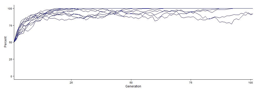
This shows an example of the output of the simulation using the default values.

If you want to actually manipulate the parameters of the simulation rather than using the default, you will need to include some numbers after evolution(. Here is a brief explanation of what each number does (everything has default values, so you can modify as many or as few of these as you want).

• First number = number of dominant alleles in the starting population (default = 100)
• Second number = number of recessive alleles in the starting population (default = 100)
• Third number = the average percentage of individuals with a dominant phenotype that will survive to a reproductive age (default = 100)
• Fourth number = the average percentage of individuals with a recessive phenotype that will survive to a reproductive age (default = 50)
• Fifth number = the number of generations it will simulate for each population (default = 100)
• Sixth number = the number of populations that it will simulate (default = 10)
• Seventh number = the number of individuals that will immigrate from a neighboring population at the end of each generation (default = 0)
• Eighth number = the number of dominant alleles in the neighboring population (default = 10, this number only maters if the seventh number is greater than 0)
• Ninth number = the number of recessive alleles in the neighboring population (default = 10, this number only maters if the seventh number is greater than 0)
• Final value = this determines the graphical output. If you enter graph=”dom” you will get the results as a graph of the percent of dominant alleles in each generation (this is the default). graph=”rec” will give you a graph of the percent of recessive alleles in each generation. graph=”surv” will give you a graph of the percent of individuals who survived to a reproductive age in each generation (i.e., recruitment).

To use these values, simply type them after evolution( and separate them by comas. For example, evolution(100,90,80,70,60,50,40,30,20,graph=”dom”) would run a simulation with a starting population of 100 dominant alleles and 90 recessive alleles (note: the sum of those two values must be a even number). On average, 80% of dominant phenotypes would survive, and 70% of recessive phenotypes would survive. It would run 60 generations per population, and a total of 50 populations. At the end of each generation, 40 individuals would immigrate from the neighboring population, and the neighboring population would consist of 30 dominant alleles for every 20 recessive alleles (i.e., 60% dominant alleles, 40% recessive alleles). When it was done, you would get a graph showing the percent of dominant alleles at the end of each generation (i.e., after selection).

Because there are default values, you can leave any parameters that you want blank, but if you skip parameters, then you need to include the commas. For example, if all that you cared about was changing the initial allele frequencies to 50 and 90, then you could enter evolution(50,90) and the program would run with 50 dominant alleles, 90 recessive alleles, and everything else set to default. If however, you only wanted to change the survivorship so that dominant phenotype never survives (0) and recessive phenotype always survived (100), you would enter, evolution( , ,0,100). You have to have those first two commas because they tell R which parameters your are actually changing. After you enter those parameters though, it knows the defaults. As a final example, suppose that you wanted the survivorship above, but you wanted to change the final output so that you could see the percent that survived each generation. Do this by entering evolution( , ,0,100, , , , , ,graph=”surv”). Anytime that you skip over a value, you need commas.

Important notes
The initial allele frequencies also determine your starting population size. Each individual has two alleles, so the total number of alleles divided by two will give you the starting population size. This means that the sum of your two allele frequencies must equal a whole number. Breeding occurs randomly and with replacement, so one parent can have more than one offspring.

It is ok if you immigrate more individuals than you have alleles in the neighboring population, because the individuals that immigrate are chosen randomly with replacement. In other words, the simulation views the numbers as ratios not true numbers (e.g., 1 and 9, 10 and 90, 100 and 900, etc, are all identical as far as the program is concerned). This only applies to the neighboring population. The initial population uses true numbers, not ratios.

Playing with the data
If you want to save your results as an excel file that you can play around with, there are several things that you need to do. First, on the top toolbar, click Session then Set working directory then Choose directory then navigate to where you would like to save your data. Next, when you run the simulation, you have to name your output. For example results <- evolution() this will name your results “results.” Once the simulation is done, type write.csv(results,”results.csv”) this will make a .csv file of your results, called “results” and save it in whatever directory you told it to (note: you can name your data and file essentially anything you want, but don’t include spaces and don’t call it “evolution”). When you open the file, the first set of columns shows the percent of dominant alleles at the start of each generation, and the second set of columns shows the percent that survived to a reproductive age in each generation. If you want the percent of recessive alleles, then just subtract the dominants from 100.

Detailed instructions and notes about the simulation

Simulation assumptions and guiding rules

• Complete dominance (i.e., homozygous dominant individuals, and heterozygous individuals behave the same way, the recessive allele is only expressed in homozygous recessive individuals)
• Discrete non-overlapping generations
• The number of offspring produced each generation is constant and always equals the initial parent population size
• Mating is random, and individuals can produce more than one offspring
• Individuals can reproduce sexually or asexually
• Mortality only occurs during recruitment into adulthood
• New immigrants are adults. Therefore, they do not undergo selection before reproducing

Simulation paramater details

Function = evolution(number_of_dominant_alleles, number_of_recessive_alleles, dominant_allele_recruitment, recessive_allele_recruitment, number_of_generations, number_of_populations, number_of_immigrants, numb_neighb_dom_alleles, numb_neighb_rec_alleles, graph)

• number_of_dominant_alleles = number of dominant alleles in the initial parent population (default = 100)
• number_of_recessive_alleles = number of recessive alleles in the initial parent population (default = 100)
  Note: number_of_dominant_alleles + number_of_recessive_alleles must equal an even number. That number divided by two = size of the parent population
• dominant_allele_recruitment = the probability that an individual with a dominant phenotype will survive to adulthood (default = 100)
• recessive_allele_recruitment = the probability that an individual with a recessive phenotype will survive to adulthood (default = 50)
  Note: dominant_allele_recruitment and recessive_allele_recruitment range from 0–100. 0 = none survive, 50 = 50% chance of survival for each individual, 100 = all survive, etc. Values must be whole numbers. Recruitment values for dominant and recessive alleles are completely independent of each other.
• number_of_generations = the number of generations that will be simulated for each population (default = 100)
• number_of_populations = the number of populations that will be simulated (default = 10)
• graph = the format of the graph that is produced (default = “dom”).
• number_of_immigrants = the number of individuals that immigrate each generation (default = 0)
  Note: immigration takes place after selection (i.e., after the formation of the new parent generation). Thus, immigrants are not under selection, but their offspring will be. Immigration does not take place until after the first round of selection.
• numb_neighb_dom_alleles = the number of dominant alleles in the neighboring population (default = 10)
• numb_neighb_rec_alleles = the number of recessive alleles in the neighboring population (default = 10)
  Note: immigrants will be randomly selected from the gene pool of numb_neighb_dom_alleles + numb_neighb_rec_alleles
• Note: words must be put in quotes.
  “dom” = graph of dominant allele frequencies against generation.
  “rec” = graph of recessive allele frequencies against generation
  “surv” = graph of survivorship (recruitment) against generation.

The following is an example showing the workflow for a run using the following parameters:

evolution(number_of_dominant_alleles=100, number_of_recessive_alleles=100, dominant_allele_recruitment=100, recessive_allele_recruitment=40, number_of_generations=100, number_of_populations=10, number_of_immigrants=10, numb_neighb_dom_alleles=50, numb_neighb_rec_alleles=100, graph=”dom”)

Note: this code could also simply be entered as evolution(100,100,100,40, 100,10,10,50,100, graph = “dom”)

This shows the basic workflow that the simulation uses.

1. It will construct a population of 100 individuals (each individual has two alleles, so population size will always = [number_of_dominant_alleles + number_of_recessive_alleles]/2).
2. It will randomly select 100 sets of two alleles (i.e., individuals).
3. It will apply the recruitment levels to each individual. In this example, all individuals with a dominant phenotype will survive, but each individual with a recessive phenotype will have a 40% chance of survival. The probabilities are run independently on each individual, so on any given run, you may have slightly more or less than 40% of recessives surviving, but the average survivorship for homozygous recessives will be 40%.
4. It will randomly select 20 alleles (10 individuals) from the neighboring population, and add them to the population of survivors, thus forming the new parent generation (if there was no immigration, this step would be skipped, and the survivors would simply be the new parent generation).
5. It will repeat steps 2–4 until it has simulated 100 generations (not including the initial parent generation). Each new run of step 2 begins with the new parent generation formed in step 4.
6. Once it has complete all 100 generations, it goes back to step 1 and starts a new population. In this case, it will make 10 populations in total.

Warning messages
Depending on the version of R you are using, and whether or not the population goes extinct part way through a simulation, you may get any of the following warning messages. Just ignore them, the simulation will still run correctly.  “package ‘ggplot2’ was built under R version 3.0.3”
“package ‘reshape2’ was built under R version 3.0.3″”No id variables; using all as measured variabls””In loop_apply(nc, do.ply): Removed   rows containing missing values (geom_path).”

General Notes

If there is no immigration, populations may go extinct part way through the simulation; however, this is less likely than it would be in a real population because the same number of offspring are produced each generation, regardless of the number individuals who survived to form the new parent population. This simplification does not adversely affect the overall patterns, and there are some real populations where the number of offspring produced is highly dependent on the number of competitors, so it is not an entirely unreasonable situation.

If there is immigration, the population make go extinct and recover multiple times during a simulation.

It may seem odd that the program selects alleles from the entire gene pool of the parent population rather than splitting the parents up into homozygous dominants, heterozygotes, and homozygous recessives, however, mathematically, both situations are identical because each allele has a 50% chance of being passed from a given parent.

For example, if your population consisted of 10 homozygous dominant individuals, 20 heterozygotes, and 10 homozygous recessives (total dominant alleles = 30, total recessive alleles = 30), then we would calculate the odds of an allele being dominant as follows:

1. The odds of having a homozygous dominant parent = 25% ([10/40]*100)
2. If a homozygous dominant parent is selected, the chance of getting a dominant allele from that parent = 100% ([2/2]*100)
3. Thus, from the product rule, the overall odds of getting a dominant allele from a homozygous dominant parent = 25% ([0.25*1]*100)
4. The odds of having a heterozygous parent = 50% ([20/40]*100)
5. If a heterozygous parent is selected, the chance of getting a dominant allele from that parent = 50% ([1/2]*100)
6. Thus, from the product rule, the overall odds of getting a dominant allele from a heterozygous parent = 25% ([0.5*0.5]*100)
7. Finally, via the sum rule, the overall odds of an allele being dominant = 50% (0.25+0.25)

Now, using the algorithm used in the simulation, where alleles are randomly selected from the gene pool without regards for homozygotes or heterozygotes, we find that there are 30 dominant alleles and 30 recessive alleles, so the chance of getting a dominant allele is 50%. So this method produces the same results as the more complicated method of including homozygotes and heterozygotes.

The actual program

Everything below this is the actual code. Simply copy it and paste into R as described above.

evolution <- function(number_of_dominant_alleles=100, number_of_recessive_alleles=100, dominant_allele_recruitment=100, recessive_allele_recruitment=50, number_of_generations=100, number_of_populations=10, number_of_immigrants=0, numb_neighb_dom_alleles=10, numb_neighb_rec_alleles=10, graph=”dom”){
require(ggplot2)
require(reshape2)

#the following simply makes a nice header row and serves as the source for the .i dataframes
c1 <- as.data.frame(cbind(c(“Parent”,rep(“Generation”,(number_of_generations)))))
c2 <- as.data.frame(cbind(c(“population”,(2:(number_of_generations+1)))))
c1 <- as.data.frame(cbind(c1,c2))
c1 <- as.data.frame(paste(c1[,1],c1[,2]))

perc_dom_alleles.i <- c1
perc_recruitment.i <- c1
for(i in 1:number_of_populations){
pop <- c(rep(1,number_of_dominant_alleles),rep(2,number_of_recessive_alleles))
pop_size <- (length(pop)/2)
prob_dom_recr <- rep(1,dominant_allele_recruitment)
prob_dom_recr <- c(prob_dom_recr,rep(2,100-length(prob_dom_recr)))
prob_rec_recr <- rep(1,recessive_allele_recruitment)
prob_rec_recr <- c(prob_rec_recr,rep(2,100-length(prob_rec_recr)))
neighb_pop <- c(rep(1,numb_neighb_dom_alleles),rep(2,numb_neighb_rec_alleles))

results.i <- as.data.frame(cbind(((number_of_dominant_alleles/(number_of_dominant_alleles+number_of_recessive_alleles))*100),NA))
colnames(results.i) <- c(“% dominant alleles”,”% recruitment”)
for(i in 1:number_of_generations){
gen.i <- NULL
#This loop will construct the population. Each individual came from a random sample of the parent population. Selection was done with replacement. 4 = homozygous dominant, 5 = heterozygous, 6 = homozygous recessive
for(i in 1:pop_size){
ind.i <- sum(sample(pop,2,F))
ind.i <- if(ind.i == 2){ind.i = 5}else{if(ind.i==3){ind.i = 6}else{if(ind.i==4){ind.i=7}}}
gen.i <- c(gen.i,ind.i)}
gen.i <- sort(gen.i)
dom.i <- length(gen.i[gen.i==5])
het.i <- length(gen.i[gen.i==6])
rec.i <- length(gen.i[gen.i==7])
#this calculates the number of homozygous dominant survivors that get recruited into the next generation
dom_surv.i <- sample(prob_dom_recr,dom.i,T)
dom_surv.i <- sum(dom_surv.i[dom_surv.i==1])
#this calculates the number of heterozygous survivors that get recruited into the next generation
het_surv.i <- sample(prob_dom_recr,het.i,T)
het_surv.i <- sum(het_surv.i[het_surv.i==1])
#this calculates the number of homozygous recessive survivors that get recruited into the next generation
rec_surv.i <- sample(prob_rec_recr,rec.i,T)
rec_surv.i <- sum(rec_surv.i[rec_surv.i==1])
#this calculates the percent of dominant alleles in the population after selection (i.e., at the start of the next generation)
perc_dom.i <- (((dom_surv.i*2)+het_surv.i)/(sum(dom_surv.i,het_surv.i,rec_surv.i)*2))*100
#this calculates the recruitment rate (as a percentage of offspring)
perc_surv.i <-  ((sum(dom_surv.i,het_surv.i,rec_surv.i))/pop_size)*100
gen_res.i <- cbind(perc_dom.i,perc_surv.i)
colnames(gen_res.i) <- c(“% dominant alleles”,”% recruitment”)
results.i <- as.data.frame(rbind(results.i,gen_res.i))
#this introduce immigrant alleles. This happens after selection and survival/allele estimates. Thus, it only affects the gene pool for the next generation
imm.i <- sample(neighb_pop,(number_of_immigrants*2),T)
pop <- c(rep(1,((dom_surv.i*2)+het_surv.i)),rep(2,((rec_surv.i*2)+het_surv.i)),imm.i)
if((perc_surv.i+number_of_immigrants) == 0){break}}
null_col <- length(results.i[,1])
null_col <- as.data.frame(cbind(c(rep(NaN,(number_of_generations+1)-null_col)),c(rep(NaN,(number_of_generations+1)-null_col))))
colnames(null_col) <- c(“% dominant alleles”,”% recruitment”)
results.i <- as.data.frame(rbind(results.i,null_col))
results.i <- round(results.i,1)
dom_a.i <- as.data.frame(cbind(results.i[,1]))
recru.i <- as.data.frame(cbind(results.i[,2]))
perc_dom_alleles.i <- as.data.frame(cbind(perc_dom_alleles.i,dom_a.i))
perc_recruitment.i <- as.data.frame(cbind(perc_recruitment.i,recru.i))}
results.i <- cbind(perc_dom_alleles.i,perc_recruitment.i)
c1 <-  c(“”,rep(“Population”,number_of_populations),””,rep(“Population”,number_of_populations))
c2 <-  c(“Generations”,1:number_of_populations,”Generations”,1:number_of_populations)
c1 <- as.data.frame(cbind(c1,c2))
c1 <- (paste(c1[,1],c1[,2]))
colnames(results.i) <- c1

if(graph == “dom”){
g.i <- as.data.frame(results.i[,1:number_of_populations+1])}

if(graph == “rec”){
g.i <- as.data.frame(results.i[,1:number_of_populations+1])
g.i <- 100-g.i}

if(graph == “surv”){
g.i <- as.data.frame(results.i[,(number_of_populations+3):ncol(results.i)])}

g.i <- melt(g.i)
col1 <- as.data.frame(cbind(rep(c(1:(number_of_generations+1)),number_of_populations)))
g.i <- cbind(col1,g.i)
colnames(g.i) <- c(“Generation”,”variable”,”Percent”)
graph <- ggplot() +
geom_line(data = g.i, aes(x = Generation, y = Percent, group = variable), color = “#000099”)

graph <- graph + theme_bw() + theme(panel.border = element_blank(), panel.grid.major = element_blank(),panel.grid.minor = element_blank(), axis.line = element_line(colour = “black”))
graph <- graph + scale_x_continuous(expand = c(0, 0)) + scale_y_continuous(limits = c(0, 100))
print(graph)
graph <- results.i
print(graph)}