In previous posts, I have explained the importance of having lots of data, but what I failed to mention was the dangers of analyzing these large data sets. You see, all real data has variation in it, and when you have a very large data set, you can usually subset it enough that eventually you find a subset that, just by chance, fits your preconceived view. Sometimes, these erroneous results arise as a deliberate form of academic dishonesty, but other times they come from honest mistakes. Regardless of their origin, they present a very serious problem because to the untrained eye (and sometimes even to the trained eye), they seem to show scientific evidence for truly absurd positions, and an enormous number of the studies and “facts” that anti-scientists cite are actually the result of this illegitimate sub-setting of large data sets. Therefore, I want to explain how and why these erroneous results arise, how scientists deal with them, and how you can watch for them so that you are not duped by research which appears to carry all the hallmarks of good science.

Note: I have split this post up into two sections. The first just explains the phenomena without going into the actual math or the gritty details of what is going on. The second half, called “Technical Notes” explains the math behind this problem. I encourage everyone to read both sections, but you can get the basic idea just by reading the first section.

I want to illustrate how this works using a totally fictitious data set. To set up this example, let’s suppose that I was working on a particular species of frog, and I wanted to know how body size effected clutch size (i.e., the number of eggs that a female lays). I examined this by measuring female frogs and their clutch sizes at 30 populations (assume that I used proper controls so that any correlation would actually show causation). Now, remember that this is a fictional data set, so to actually generate it, I used the statistical program R to generate 30 sets of random data. Each set contained the body size and clutch size for 50 individuals. For body size, the computer randomly selected a number between 1 and 1,000 (inclusive), and for clutch size it selected a random number between 1 and 500 (inclusive). So I got “measurements” from a total of 1,500 “individuals.” When I put all of those individuals together, I got the figure below.

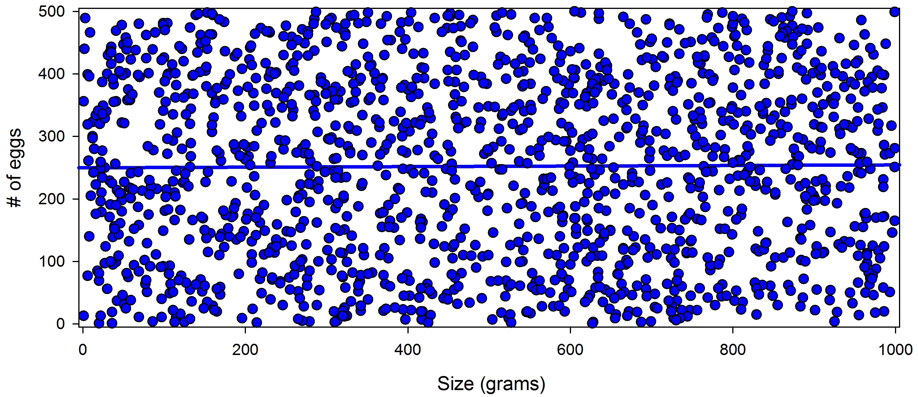
Figure 1: A comparison of body size and clutch size for my fictional data set (data were randomly selected). As expected, there is no relationship between our variables. You can see this in the flat trend line.

As we would expect, there is no relationship between body size and the number of eggs that a female laid. This is what we should find since the data came from a random number generator. In this case, it is pretty obvious to just look at the trend line and see that there are no relationships, but scientists like to actually test things statistically because statistics give us an objective way to tell determine whether or not there are any relationships. For these data, the appropriate test is what is known as a Spearman rank test. Running this test produces a P value of 0.7615. I explain P values more in the Technical Notes section, but for now, just realize that for most scientific studies, anything less than 0.05 is considered significant. So when you see a scientific study state that it found a “significant difference” or “significant relationship” it usually means that the P value was less than 0.05.

So far, everything is as it should be: there is no significant relationship. However, watch what happens when I subset the data. This time, I’m going to display each population separately.

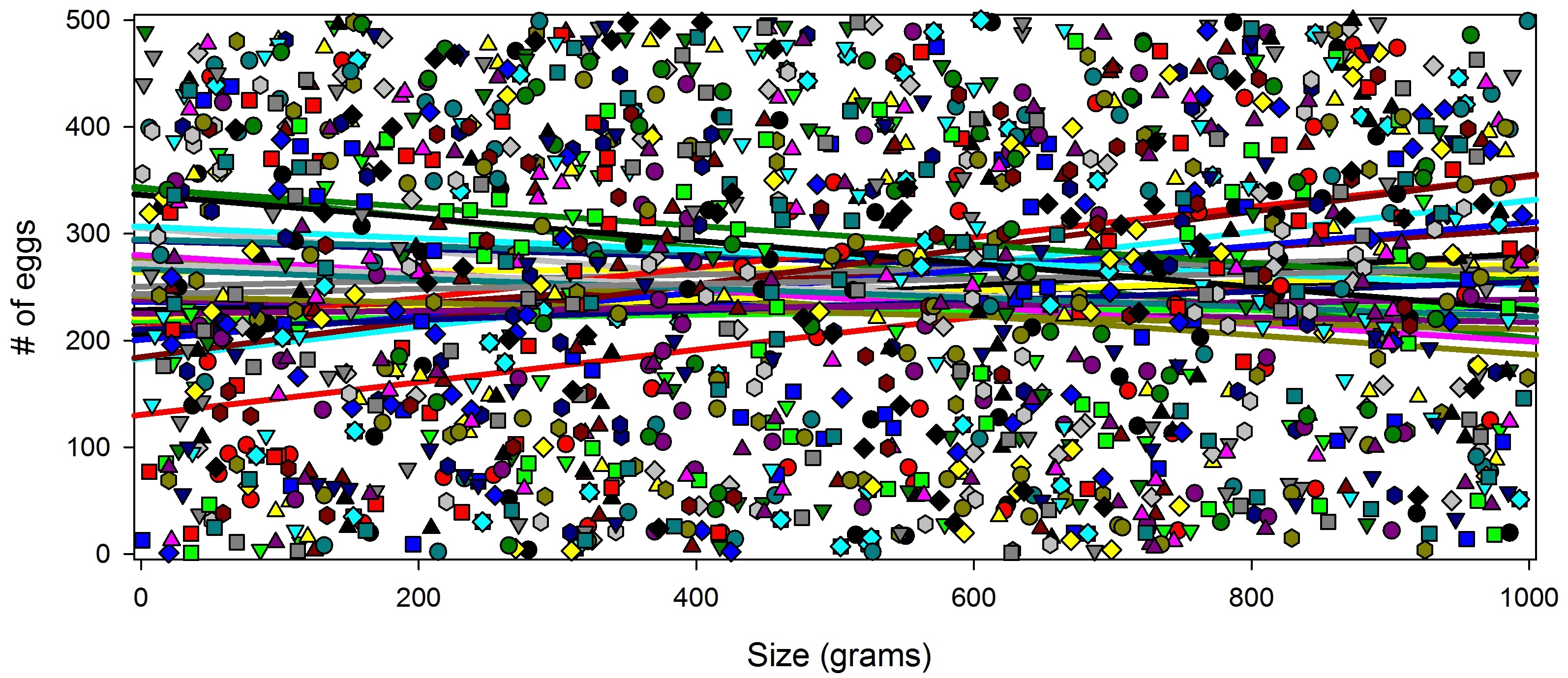
Figure 2: These are the same data as figure 1, but the data have been subset by population so that each population is now shown separately (note: the data are fictional and were randomly generated).

That’s obviously a bit of a mess to look at, but a few of those lines appear to be showing a relationship, and when we run a Spearman rank test on each subset, we find that populations 2, 19, and 23 all had a significant positive relationship between frog size and clutch size!

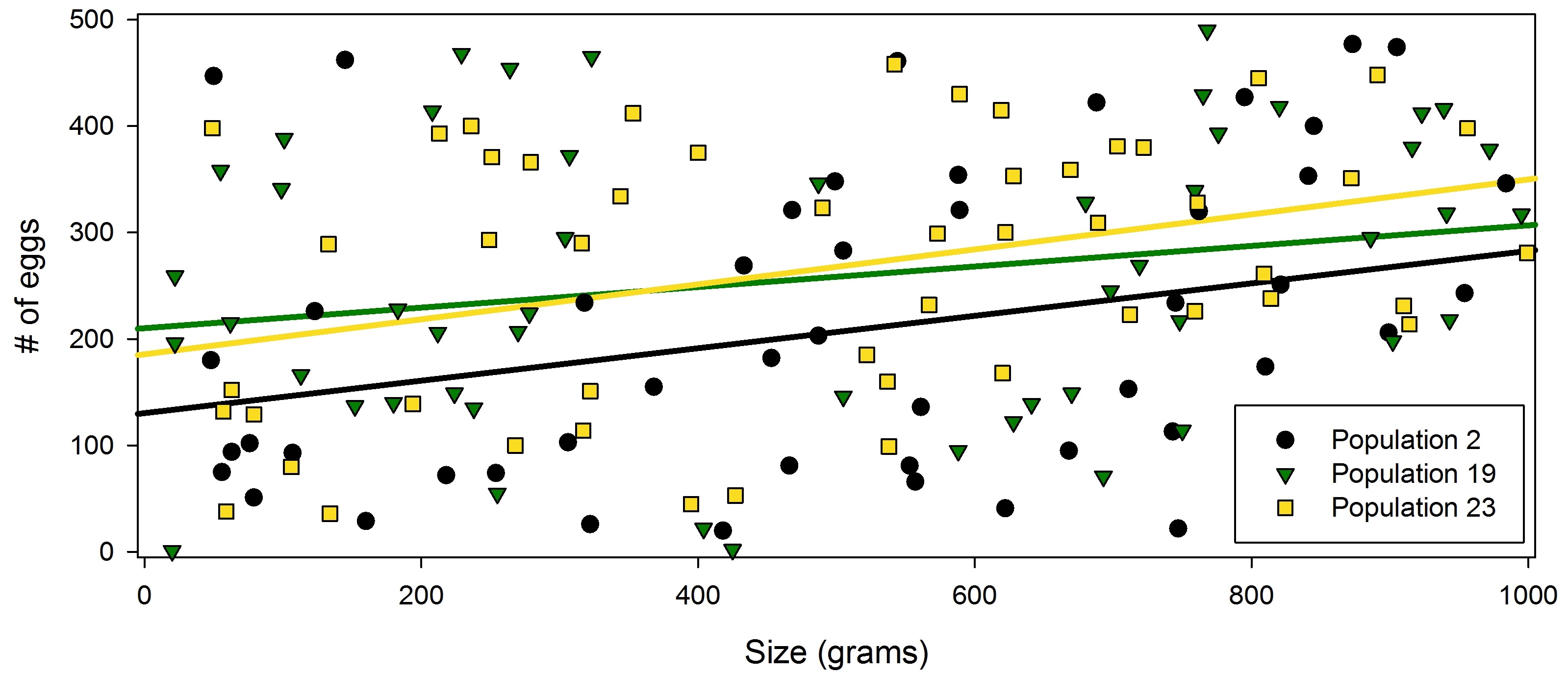
Figure 3: This just shows the data for populations 2, 19, and 23. All three of them had significant positive relationships. (note: the data are fictional and were randomly generated)

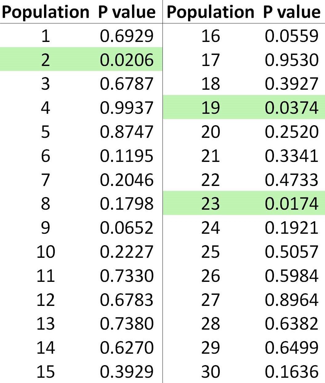
Table 1: P values for all 30 fictional populations. Anything less than 0.05 was considered statistically significant. The three significant populations have been highlighted.

Unless you already have a good understanding of probability theory, this should surprise, shock, and disturb you. We know that there is not actually a relationship between these two variables because I randomly selected the numbers, yet three of our populations are showing significant relationships! What is going on here? Are all statistics part of a massive lie by the government/big pharma/Monsanto designed to deceive us into allowing them to poison the food supply, fill our children with toxins, neuter our pets, and inject us with mind controlling chemicals!? Hardly.

The reality is that this is a well-known statistical fluke known as a type 1 error. This type of error occurs anytime that you incorrectly conclude that there is either a relationship between variables or a difference between groups (see Technical Notes for details). This is simply an unavoidable byproduct of the law of large numbers. Because of natural variation in data, you will inevitably get erroneous results from time to time. Fortunately, there are ways to control this type of error when you are working with subgroups of large data sets (see Technical Notes). The problem is that sometimes studies that did not use these controls manage to make it through the peer-review process, and the media and general public have a panic over “results” that are actually just statistical outliers.
The breeding habits of frogs rarely make the news, so to illustrate this problem, imagine instead that my data set was looking at the side effects of a vaccine, or, perhaps it was looking for relationships between GMO consumption and neurological problems among different age groups. You can no doubt envision the headlines, “GMOs are dangerous for 10-15 year olds,” “New study proves that GMOs are dangerous,” etc. The problem is that, in this example, we know that the results are spurious. They are just from random chance, but to the untrained eye, they appear to show significant relationships for certain subgroups.

My data set is fictional, but this happens with real data and it causes all manner of problems. A great example of this occurred last year in a highly publicized paper called, “Measles-mumps-rubella vaccination timing and autism among young African American boys: a reanalysis of CDC data.” The headlines from the media and anti-vaccers were predictable, “New Study Finds A 340 Percent Increased Risk Of Autism In Boys Who Receive MMR Vaccine On Time” (from Collective-evolution), “MMR vaccines cause 340% increased risk of autism in African American infants” (from Natural News), etc. When we look at the actual study though, we find that it is fraught with problems. The one that I want to focus on is sub-setting. The authors took a data set of several hundred children, then subset it by race, then subset those subsets by sex, then subset those subsets by age at injection. So we now have lots of subsets, and out of all of those subsets only the group of 36 month old African American males was significant, and the authors failed to control their type 1 error rate. Is the problem with this approach obvious? It should be. This is exactly the same thing that happened with my fictional frog data. Once you subset the data enough, you will eventually find some tiny subset that just by chance appears to support your position.

Further, even if this result wasn’t simply a statistical anomaly, the “news” articles about it are still a clear example of a sharpshooter fallacy, because 36 month old African American boys was the only group that showed a significant relationship. The headlines should have said, “MMR vaccine safe for everyone except 36 month old African American males.” Males of all other races = no relationship. African American males of other age groups = no relationship. African American girls of any age group = no relationship, etc. This one, tiny subgroup is the only group with a significant difference, making this is a classic type 1 error. Fortunately, I was not the only one who could spot the problem with this paper, and multiple scientists quickly pointed out its numerous flaws, ultimately resulting in a speedy retraction by the journal.

Now that you understand how this works, you should be able to spot this problem in lots of pseudoscientific papers. For example, many of the papers that I have read on homeopathy used lots of different measurements for the exact same treatment without controlling the type 1 error rate, and out of the 20 types of measurements that they used, one happened to show a significant improvement. When you get results like that, you shouldn’t conclude that homeopathy works. Rather, you must acknowledge that 19 out of 20 measurements showed no improvement, therefore, the one that did show an improvement was probably a statistical outlier.

Before delving into some fun mathematical details, I want to discuss one last case where this occurs. Everything that I have talked about so far has been either a deliberate manipulation of the data, or a mistake by the researchers in which they did not use the correct statistical methods. There is, however, another way that you get these spurious results without any mistakes or deception by the researchers. Let’s go back to my frog populations again, but this time, imagine that instead of studying all 30 populations, I just studied population #2 (assume that I got the same data as I did in my simulation). There was no dishonest or biased reason that I chose that population. It was just the one that was available for me to examine. Studying that population would, however, give me an erroneous, significant result, but because that was the only population that I studied, I would have no way of knowing that the result was incorrect. Even if I did everything correctly, designed a perfect project, and used the appropriate statistics, I would still get and publish a false result without ever knowing that I was doing so.

It’s important to understand this because this problem happens in real research. Papers get published by good, honest researchers saying that a drug works or a treatment is dangerous when, in fact, the results were simply from statistical anomalies. This is one of the key reasons that scientists try to replicate each others research. Suppose, for example, that 29 other researchers decided to try to replicate my results by studying the other 29 frog populations. Now, we would have 30 papers, 3 of which say that body size affects clutch size and 27 that say that there is no relationship. This lets us do something called a meta-analysis. This is an extremely powerful tool where you take the data from several studies and run your analyses across the whole data set. You can think of this like taking all the individual populations of frogs (Figure 2) and combining them into one massive population (Figure 1; the math is actually significantly more complicated than that, but that’s the basic idea). This method is great because it lets us see the central trends, rather than the statistical outliers. Also, remember that the law of large numbers tells us that the calculated value of large data sets should be very close to the true value. In other words, large data sets should give us very accurate results.

One of my favorite meta-analyses was published last year, and looked at the relationship between the MMR vaccine and neurological problems like autism. I cite this study a lot on this blog, but that is because it provides such powerful evidence that vaccines are safe. It combined the results of 10 different safety trials, giving it an enormous sample size of over 1.2 million children (feel free to rub that in the face of any anti-vaccer who says that the safety of vaccines hasn’t been tested). With that large of a sample size we expect to see true results, not statistical outliers. So the fact that it found no relationships between vaccines and autism is extremely powerful evidence that vaccines do not cause autism.

You can find these meta-analyses for lots of different topics, and they are crucially important because they have such large sample sizes. You can, for example, find scattered papers from individual trails that found significant improvements using homeopathy, but you can also find plenty of papers showing that homeopathy did not work for many trials, and it can be difficult (especially as a layperson) to wade through that flood of information and determine what is actually going on and which studies you should trust. That’s the beauty of meta-analyses, they comb through the literature for you and give you the central trends of the data. To be clear, I am not advocating that you blindly accept the results of meta-analyses. You still need to carefully and rationally examine them, just like you do every other paper, but, they often do a much better job of presenting true results.

In conclusion, I would like to give several pieces of advice to those of you who are interested in truly informing yourself about scientific topics (as I hope you all are). First, take the time to learn at least the basics of statistics. Learn how the tests work, when to use them, and how to interpret their results. I personally recommend studying the Handbook of Biological Statistics. It’s a great website that does a fantastic job of introducing a lot of statistical tests in a way that most people can understand. Second, watch out for these type 1 errors. Learn the methods that we use to control them, and when you’re reading the literature, make sure that the authors used those controls. Finally, look for the meta-analyses. They are one of our most powerful tools, and they can really help you sort through the tangled mess that is academic literature.

Technical Notes
P-values and alphas
In statistics, you are generally testing two hypotheses: the null hypothesis and the alternative hypothesis. The null hypothesis usually states either that there is no association between the variables you are testing or that there are no differences between your groups. The alternative hypothesis states the opposite. It states that there is a significant relationship/difference. The P value is the probability of getting the results that you got if the null hypothesis is actually true. So if you are comparing the average value of two groups (group 1 mean = 120, group 2 mean = 130), and you get a P value of 0.8, that means that if there is no significant difference between those groups (i.e., the null hypothesis is true) then, just by chance, you should get the result that you got 80% of the time. So most likely, your “difference” of an average of 10 is just a result of chance variation in the data. In contrast, if you get a P value of 0.0001, that means that if the null hypothesis is actually true, you should only get your results 0.01% of the time. This makes it very likely that your difference is a true difference, rather than just a statistical anomaly. Thus, the smaller your P value, the more confidence you have in your results.

It’s important to note that you can never prove anything with statistics. You can show that there is only a 0.0000000000000000000000000000000000000000000000000001% chance of getting your result if the null is true, but you can never prove anything with 100% certainty.

To objectively determine whether or not there is a significant relationship/difference, you compare your P value to a predetermined significance value called alpha. Generally speaking, you use an alpha of 0.05, but sometimes other alphas are used, especially 0.01. So, if your calculated P value is less than your alpha, you reject the null hypothesis. In other words, you conclude that your result is statistically significant. Whereas if your P value is equal to or greater than your alpha, you fail to reject the null hypothesis (this is not the same thing as accepting the null, but that’s a conversation for another post). Importantly, your alpha must be determined ahead of time, and you are not allowed to cheat. If your alpha is 0.05 and your P value is 0.051, you cannot claim significance or talk about your results as if they were significant. This is, however, another case where meta-analyses come in handy. Sometimes, there is a significant result, but your sample size was too small to detect it, so by combing your data with the data from other studies, you can boost the sample size and reveal a trend that was not visible just by looking at your data.

Type 1 and type 2 errors
A type 1 error occurs anytime that you reject the null hypothesis when the null hypothesis was actually correct. Remember, P values are the probability of getting your results if the null hypothesis is actually true. So, if you have an alpha of 0.05, then a P value of 0.049 will be significant, but you should get that result just by chance 4.9% of the time. If you think back to my fictional frog data, this is why some of the populations were significant. Because I had 30 populations, I expected that just by chance some of them would happen to have body sizes that produced a P value less than 0.05.

Now, you may be thinking, “well why not just make the alpha really tiny, that way you almost never have a type 1 error.” The problem is that then you get a type 2 error. This occurs when you fail to reject the null hypothesis, but the null hypothesis was actually incorrect. In other words, there was a significant relationship, but you didn’t detect it. So if, for example, we used an alpha of 0.00001, we would have an extremely low type 1 error rate, but we would almost never have any significant results. In other words, almost all of our studies would be type 2 errors. So the alpha level is a balance between type 1 and type 2 errors. If it’s too large, then you have too many type 1 errors, but if it is too small, then you have too many type 2 errors.

Family-wise type 1 error rates
The family-wise type one error rate is basically what this whole post has been about. When you are testing the same thing multiple times, your actual type 1 error rate is not the standard alpha. Think about it this way, if you did 100 identical experiments and the null hypothesis was true, we would expect, just by chance, that five of the experiments would have a P value of 0.05. This is, again, what happened with the frog data. So you need a new alpha level that accounts for the fact that you are doing multiple tests on the same question. This new alpha is your family wise type 1 error rate.

There are several ways to calculate the modified error rates, but one of the most popular is the Bonferroni correction. To do this, you take the alpha that you actually want (usually 0.05) and divide it by the number of tests you are doing. This results in a 5% chance that any of your results will have a P value of 0.05 if the null hypothesis is correct. So, if we apply this to my fictional frog data, I had 30 populations, so my corrected alpha is 0.05/30 = 0.00167. So, for any of my populations to show a significant relationship, they must have a P value less than 0.00167. My lowest P value was, however, 0.0174. So, now that done the correct analysis and have properly controlled the family-wise error rate, we can see that there are no significant relationships between body size and clutch size, which is, of course, what we should see since these data were randomly generated. This is why it is so important to understand these statistics: if you don’t control your family-wise error rate, you are going to get erroneous results.

It’s worth mentioning that the standard Bonferroni correction tends to slightly inflate the type 2 error rate, so I (and many other researchers) prefer the sequential Bonferroni correction. This works the same basic way but with one important difference: rather than comparing all of your P values to alpha/# of tests, you compare the lowest P value to alpha/# of tests, the second lowest P value to alpha/(# of tests – 1), the third lowest P value to alpha/(# of tests – 2), etc. You keep doing this until you reach a P value is that is greater than or equal to the alpha you are comparing it to. At that point, you conclude that that test and all subsequent tests are not significant. So, for my frog data, we are done after the first comparison because even my lowest P value was greater than 0.00167, but let’s suppose instead that my four lowest P values were: 0.0001, 0.0002, 0.0016, and 0.003. First, we compare 0.0001 to 0.05/30 = 0.00167. Since 0.0001 is less than 0.00167, we reject the null. Next, we compare 0.0002 to 0.05/29 = 0.00172. Again, reject the null. Next, we compare 0.0016 to 0.05/28 = 0.00179. Again, reject the null. Then, we compare 0.003 to 0.05/27 = 0.00185. Now, our P value is greater than our alpha, so we fail to reject the null for this test and for all 26 other tests that produced larger P values.

A final way to deal with this problem of multiple comparisons (and really the best way) is to design your experiment such that you can use a statistical test that incorporates your subsets into the model and accounts for the fact that you are making several comparisons. Entire books have been written on this topic, so I won’t go into details, but to put it simply, some tests (like the ever popular ANOVA) allow you to enter different groups as factors in your analysis. Thus, the test makes the comparisons while controlling the error rate for you. Again, I want to impress upon you that if you want to be able to understand scientific results, you need to at least learn the most common statistical tests and how and when they are used. This is fundamental to understanding modern science. If you don’t understand statistics, you’re not going to be able to understand scientific papers, at least not in a way that lets you objectively assess the authors’ conclusions.

Other posts on statistics:

• Basic Statistics Part 1: The Law of Large Numbers
• Basic Statistics Part 2: Correlation vs. Causation
• Basic statistics part 4: Understanding P values