From time to time, I get directed to an article titled “One Hundred Arguments Against Vaccines” which was written by Natural Health Warriors and is nothing more than a Gish Gallop of anti-vaccine tropes. I have been loath to address this article because, quite frankly, I don’t really feel like spending several days debunking this nonsense. Nevertheless, given the frequency with which I encounter this article, I suppose it would be worthwhile to write a rebuttal. So here it is. Those of you who read this blog know that I like to pontificate, and I struggle with brevity, but given that I have 100 arguments to deal with, I will attempt to be terse. Many of these are arguments that I or others have dealt with in more detail elsewhere, so when relevant, I will link to those articles in case you want a more thorough refutation. Also, several of these arguments are nearly identical to each other, so I have grouped those and written a single response to all of them (note: all of the bad arguments are direct quotes from the Natural Health Warriors post [including the caps lock]).
 As you read through this, I want you to pay very careful attention to an important difference between the original article and my rebuttal. Namely, the “sources” for the original were almost entirely quack websites like Natural News, Whale.to, Info Wars, etc. Indeed, there were only citations to a few (I think three) peer-reviewed papers in the entire post, and most of them weren’t about vaccines. In contrast, I constantly back up my claims with peer-reviewed studies or statistics from reputable groups like the CDC and WHO. I may direct you to blogs for more detailed explanations, but I always back up factual claims with proper sources. On that note, if you disagree with my arguments, please do not bother to post unless you include references to the peer-reviewed literature. To be blunt, I do not give a crap about your anecdotes, gut feelings, opinions, or “hours of research.” Unless you can back up your position with properly conducted studies, your position is invalid.
Bad Argument #1). “NO vaccine is 100% safe.”
True…but neither is measles, polio, rubella, etc. Vaccines are a basic exercise in risk assessment. They have been tested over and over again, and their risks are extremely small. Conversely, the consequences of the diseases that they prevent are horrible. For example, Clemens et al. (1988) found that the introduction of the measles vaccine reduce death rates by 57%. In short, vaccines are far safer than the diseases that they prevent. For more details (and sources) see this post.
Bad Argument #2). “NO vaccine is 100% effective.”
I could say the same thing about seat belts, car seats, condoms, helmets, parachutes, sunscreen, etc. The fact that something isn’t 100% effective clearly doesn’t mean that we shouldn’t use it (i.e., this argument is logically inconsistent). Also, do you know what is 0% effective? Not vaccinating! (more details here).
Bad Argument #3). “ALL vaccines have severe life-threatening side-effects. Any ‘immunity’ gained from a vaccine is short term only.”
Again, life threatening side-effects from vaccines are extremely, extremely rare. For example, life threatening responses to the MMR vaccine occur in roughly 1 in 1,000,000 cases, and they are usually allergic reactions, which can be treated instantly since you are already at a medical facility. So deaths from vaccines are almost unheard of. In contrast, measles kills 1 out of every 1,000 people that it infects, resulting in thousands of deaths every year. Further, for some vaccines, immunity does last for a long time (Hammarlund et al. 2003; Jokinen et al. 2007), and even when it is short lived, vaccines are still better than having no protection at all. Further, in some cases natural immunity also isn’t life long (Wendelboe et al. 2005).
Bad Argument #4). “There are no long term studies that have been done on the effects of vaccination.”
Define “long term”? Is “long term” 5 years? 10 years? 20 years? Without a clear definition of “long term” this criticism is vague to the point of uselessness. There have been several studies that have looked at vaccine effects over multiple years (Idbal et al. 2013; Ferris et al. 2014; Vincenzo et al. 2014), but “long-term” really needs to be defined beforehand. Also, realize that studies over several decades are inherently problematic because it becomes almost impossible to control all of the variables. Finally, the fact that there aren’t any studies over a 30 year period in no way shape or form justifies that conclusion that vaccines are dangerous (that would be an argument from ignorance fallacy).
Bad Argument #5). “Vaccine safety trials are only carried out on healthy babies, children and adults yet once approved, they are given to everyone – healthy or not.”
Actually, there are quite a few illnesses and disorders (such as being immunocompromised) that will prevent you from getting a vaccine (please see the CDC recommendations). Further, there are studies that look specifically at how people with various medical conditions respond to vaccines. For example, Kramarz et al. (2000) examined the effects of the flu vaccine on children with asthma.
Bad Argument #6). “Vaccine safety trials are paid for by the very people who make the vaccines, so there is no possibility of the information being unbiased or truthful.”
First, there are many safety trials that were not funded by vaccine manufactures (more details here). Second, let’s not forget that many of the people/sites that oppose vaccines make a lot of money from doing so (including sites that this article cites), so this argument is logically inconsistent (more details here and here). Finally, “no possibility,” really? The fact that someone works for a pharmaceutical company does not automatically mean that they are corrupt.
Bad Argument #7). “Unvaccinated children are much healthier than vaccinated children.”
This one links to a statistically invalid, self-reported survey. Basically, they polled their audience of anti-vaxxers and asked them to rate their children’s health, and (big surprise) they said that children without vaccines were healthier. This survey is completely illegitimate. It lacks all of the proper controls and randomizations that would be necessary for it to be valid. It is no different than polling people as they exit Whole Foods and asking them to rate their health when they eat organic vs. non-organic food. Of course they are going to say that they feel better when eating organic, that’s why they are shopping there! In contrast, a properly conducted, peer-reviewed study (Schmitz et al. 2011) compared the health of vaccinated and unvaccinated children, and the only difference was that unvaccinated children had vaccine preventable diseases significantly more often than vaccinated children. Further, Grabenhenrich et al. (2014) found that asthma rates are actually lower among the vaccinated. So in reality, vaccinated children are much healthier.
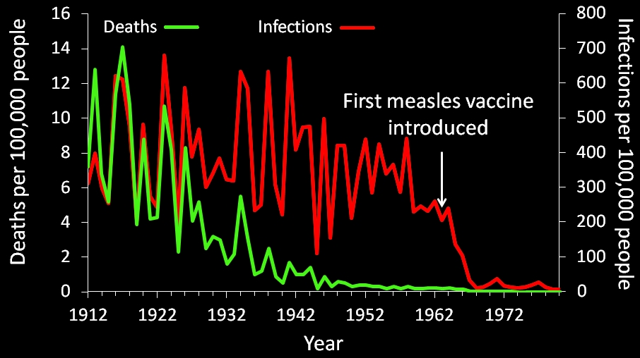
US measles infection and mortality rates prior to and following the introduction of the measles vaccine. Notice that although death rates had decreased prior to vaccines, infection rates had not (sources are available at the end of this post).
Bad Argument #8). “Vaccination is NOT responsible for the decline in infectious diseases.”
No, actually it is. I dealt with this argument in detail here, but in short death rates had declined prior to vaccines, but actual infection rates had not. Further, numerous studies have found that disease rates declined sharply following the introduction of vaccines (Clemens et al. 1988; Adgebola et al. 2005; Richardson et al. 2010), and diseases have a nasty habit of returning when vaccine rates drop (Antona et al. 2013; Knol et al. 2013).
Bad Argument #9). “The polio vaccine of the 1950’s and 60’s was contaminated by the SV40 virus which is now confirmed to have caused cancer in many people who had received the vaccine. New viruses are being discovered all the time, so it’s a matter of Russian roulette on when such a virus will sneak into another vaccine.”
This argument boils down to, “the medical technologies of the 1950’s and 60’s were inadequate, therefore the medical technologies today are.” That is just silly. Standards and techniques have come a long way since then. This argument is like saying, “the first plane only flew a few feet, therefore modern transcontinental flights are dangerous.” Also, SV40 doesn’t cause cancer (you can find a lengthy explanation and sources here).
Bad Argument #10).“The cells of an aborted human fetus was used to make the rubella vaccine, which is part of the MMR vaccine.”
This is an appeal to emotion fallacy. Also, just to be clear, there are no aborted cells in the vaccines, and no new fetuses are being aborted for vaccines. The cells are simply used to culture the virus (details here).
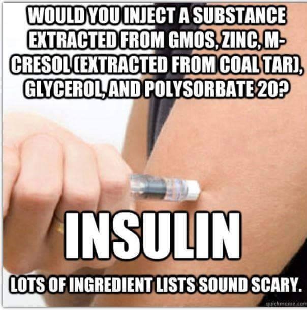
Image via Refutations to Anti-Vaccine Memes
Bad Argument #11). “Cow cells, monkey cells and chick embryo cells are all found in various vaccines – how can anyone really know the long term effects of injecting this foreign DNA into a 6 week old baby’s body?”
This is both an appeal to emotion fallacy and an argument from ignorance fallacy. Also, none of those things are actually in the vaccines. Some vaccines contain cell proteins, but they do not contain the cells themselves (here’s a list of vaccine ingredients). More importantly, there is no reason to think that these cell proteins are dangerous, especially when thousands of studies all say that vaccines are safe. Also, realize that chemically, the DNA of all organisms is the same (it’s all deoxyribonucleic acid), and the foreign DNA isn’t going to get incorporated into your child’s genetic code (that only happens in comic books; more details here).
Bad Argument #12). “Add some heavy metals, antibiotics and preservatives and you have a toxic cocktail called a vaccine.”
This is yet another appeal to emotion fallacy (are you detecting a theme here?). Further, it ignores the fact that the dose makes the poison. The “toxic” chemicals in vaccines are present in extremely low doses, and they are perfectly safe at those concentrations (details here).
Bad Argument #13). “Oh, and don’t forget to add some GMO’s to the above as well!”
(sigh) Again, this is an appeal to emotion fallacy. Just because something sounds gross doesn’t mean that it is actually bad. You have to actually provide evidence that GMOs in vaccines are dangerous. Also, don’t forget that the life-saving drug known as insulin also comes from a GMO.
Bad Argument #14). “PHARMACEUTICAL COMPANIES CANNOT BE TRUSTED! They have proven over and over again that they are only in it for the money.”
This is a guilt by association fallacy (i.e., whether or not the companies are ethical has no bearing on whether or not vaccines work). Look, no one is saying that pharmaceutical companies are angelic, benevolent entities that are trying to bring about world peace and ensure that everyone has a unicorn for a pet. They are for profit companies which, by definition, means that their primary goal is money. I’m not contesting that. Also, like essentially all big companies, they will behave unethically for the sake of money, but accepting vaccines isn’t about trusting pharmaceutical companies, it’s about trusting science, and the scientific evidence says that vaccines are safe and effective. Also, please note that there are plenty of vaccine studies that aren’t affiliated with pharmaceutical companies, and vaccines aren’t actually worth that much to pharmaceutical companies (details here).
Bad Argument #15). “An Italian court has ruled that MMR was the cause of autism in this man’s case.”
Your point is…? Judges and lawyers aren’t science experts, and even if they were, the fact that they said that the vaccine caused the autism does not prove that the vaccine caused the autism. This is a blatant inappropriate appeal to authority fallacy. Further, this ruling was later overturned. The “link” between autism and vaccines has been tested dozens of times. We have conducted a massive meta-analysis with over 1.2 million children (Taylor et al. 2014); we have looked specifically at children who are at a high risk of autism (Jain et al. 2015); we have even examined how vaccines affect the brains of rhesus macaques (Gadad et al. 2015), and we have always gotten the same result: vaccines do not cause autism. If you still think that vaccines cause autism, then you are willfully ignorant of reality (I discussed the literature at length here and explained why there are so many anecdotes of autism and vaccines co-occurring here).
Note: none of the three studies that I cited were funded by pharmaceutical companies, in fact, the monkey study was funded by anti-vaccers! Several of the authors of Jain et al. 2015 do work for the UnitedHealth Group and its subsidiaries, but they are not involved in the manufacturing of vaccines).
Bad Argument #16). “In New Zealand a fully vaccinated child in 1961 would have received 12 vaccines for four diseases (four jabs and three sips) up until the age of five. The current vaccine schedule includes 11 injections for 10 diseases by age four. This will continue to increase as the pharmaceutical companies realize they can make more money if they inject our children with more vaccines.”
First, let’s do some basic math. Twelve divide by 4 is 3, and 11 divided by 10 is 1.1. So in 1961, it took 3 vaccines per disease, whereas now it takes 1.1 vaccines per disease (assuming that their numbers are even true, I didn’t check). In other words, the number of vaccines per disease is decreasing. If this was truly all about the money, we would expect the exact opposite, there should be more injections per vaccine, not fewer. Further, the reason that there are more injections today is because today children are protected against more diseases, which is a good thing! This argument is no different from complaining that cars today have more airbags than they did in the 60s!
Bad Argument #17). “Herd immunity by means of vaccination is a LIE the pharmaceutical companies use to make parents feel bad for not vaccinating their children.”
No it’s not., It is an empirical fact which can easily be calculated and simulated (see here, here, and here), and has been experimentally demonstrated numerous times (Monto et al. 1970; Rudenko et al. 1993; Hurwitz et al. 2000; Reichert et al. 2001; Ramsay et al. 2003).
Bad Argument #18).”Vaccines are regularly being withdrawn from the market due to adverse reactions.”
To check the facts on this, I went straight to the FDA website and looked at the vaccine recalls over the past 5 years. There have only been nine, and all of them were for particular batches, not the entire vaccine. In fact, none of them were because the vaccine itself had been found to be dangerous. One was simply that there was an error on the insert package, another was that some vials were cracked, and a third was that the batch had been shipped to the wrong country. Most of the recalls were because the company had preemptively recalled the batch because that particular batch tested below their standards (no adverse effects had been document). In fact, only two of the recalls directly mentioned potential adverse health effects, and both of those were because of problems with the vials, not because of problems with the vaccines themselves. So, rather than showing that vaccines are dangerous, these recalls show an incredibly high level of quality control. Finally, let’s not forget that any product that is made on such an enormous scale is occasionally going to have defects, but the defects are extraordinarily rare compared to the volume that is being produced.
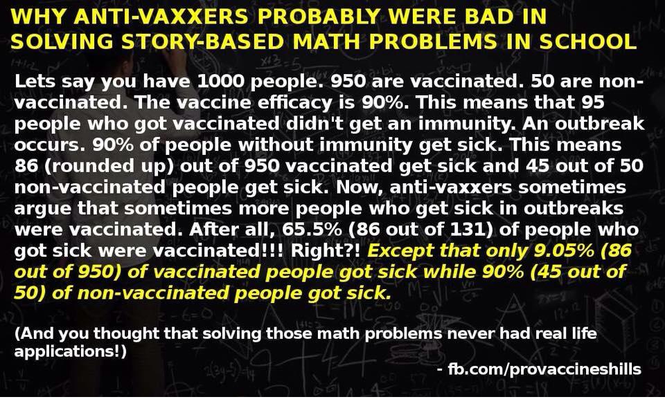
Bad Argument #19). “In New Zealand, 65% of people who contracted whooping cough in 2012 were vaccinated.”
Bad Argument #20). “Most children who catch measles were already vaccinated.”
Anti-vaccers apparently suck at math. It is true, that in raw numbers the majority of infected people were vaccinated, but that is because the majority of the population was vaccinated. So, when you look at the actual percentages (i.e., infection rates), you find that the unvaccinated have far higher disease rates than the vaccinated (I explained the math in more detail here).
Bad Argument #21). “Even ex-vaccine developers are coming out and exposing the lies that the vaccination industry is based on.”
This links to an “interview” with someone who claims to be an ex-vaccine developer (pseudonym: Dr. Mark Randall), but the interview contains all the usual anti-vaccine tropes, as well as clearly unfactual statements, and numerous conspiracy theories (such as the WHO being involved in depopulation efforts). Finally, realize we are given no actual information about this person. We don’t know who he is, where he worked, what his credentials are, or if he actually even exists. We are just supposed to take the interviewer’s word for everything, but the interviewer is not a credible, well-respected journalist, he (Jon Rappaport) is a conspiracy theorist who also writes posts about mind control, HIV conspiracies, etc. In other words, there is absolutely no reason to trust anything in this “interview.” Extraordinary claims require extraordinary evidence, and this just doesn’t cut it.
Bad Argument #22). “The swine flu vaccine caused an increase of narcolepsy cases in children recently.”
For once, the claim is actually true, but it’s not nearly as bad as it sounds. First, this was a regional phenomena (not a global one) and appears to be an interaction between the vaccine and an underlying genetic issue. Second, I reiterate that vaccines do admittedly have side effects (as do all real medical treatments), but they are very rare (see #1). In this case, the three estimated rates of vaccine induced narcolepsy were 1 in 12,000, 3 in 100,000 and 1 in 100,000, all three of which are extremely low.
Bad Argument #23). “At least one death in NZ has been linked to the Gardasil vaccine.”
Bad Argument #24). “…and four more deaths from Gardasil in India.”
This is a post hoc ergo propter hoc fallacy. Just because A happened before B does not mean that A caused B, so the fact that someone died after taking the vaccine does not prove that the vaccine killed them. For the NZ case, this person received the vaccine and died several months later, resulting in the mother being convinced that it was the vaccine, but there is absolutely no way to prove that. In fact, the very article that this post cited contains several other completely plausible explanations for the death.
The article that was cited for the India deaths was more vague, making it hard to refute directly, but I did find this report of seven deaths following Gardasil in India (I presume that the four deaths being discussed are included in those seven), and, importantly, none of those deaths appear to be related to the vaccine. “One girl drowned in a quarry; another died from a snake bite; two committed suicide by ingesting pesticides; and one died from complications of malaria.” So unless you think that the vaccine caused a snake bite, that leaves just two deaths, and the Indian Council of Medical Research concluded that neither of them were caused by the vaccine.
Bad Argument #25). “Homeless people died after being paid £1-2 to participate in a vaccine trial.”
This claim included a link to an article in the Telegraph, and I have been able to find very little information beyond what is in that article. From what I have found, it does appear that there may have been some unethical practices by certain people involved, but that does not prove that all of the scientists/doctors involved in vaccine testing are unethical (that would be a hasty generalization fallacy/guilt by association fallacy). Further, the guilty parties were caught and dealt with, and the study was stopped. Also, it is not clear that the people who died actually died as a result of the vaccine (they may have died for completely different reasons). Finally, this was an experimental trial of a new vaccine, so it doesn’t provide evidence that the vaccines that passed their safety trials are dangerous.
Bad Argument #26). “Since the 1980’s, vaccine manufacturers in the USA have been protected from lawsuits following vaccine injury.”
First, what’s your point? What exactly do you think this proves? Second, you cannot sue them directly, but you can get money through the National Vaccine Injury Compensation Program (NVICP), which is essentially a no fault system that does not require proof that the vaccine was responsible. In other words, you can get money for essentially any potentially plausible claim of vaccine injury even if the vaccine was in no way at fault (more details about the NVICP here and here).
Bad Argument #27). “Vaccination is being used to REDUCE fertility and reduce the worldwide population.”
The logic of this one is so bad it makes my soul cry. Here’s the deal: various vaccine manufacturers have experimented with birth control vaccines (i.e., a vaccine which is designed solely to prevent pregnancy), just as they have experimented with pills, IUDs, and other forms of contraceptives. This does not mean that the vaccines that you receive reduce fertility, nor does it mean that companies are trying to reduce the world’s population. This argument is no different from saying, “the same company makes birth control pills and aspirin, therefore aspirin reduces fertility and is a secret plot to depopulate the planet” (here is their “source“).
Bad Argument #28). “The pro-vaccine movement openly admits that it is willing to sacrifice some lives in order to ‘save’ many. I’m not willing to risk that my child is that one that will get sacrificed due to vaccine damage.”
First, the risk to your child is extremely minimal. No one is asking your kid to be a tribute for District 12. Second, if everyone was as selfish as you, then disease rates would skyrocket and the risk to your child would be much higher than it currently is. Further, let’s not forget that your child is much safer with a vaccine than without it. So this argument is both selfish and ignorant (see Gangarosa et al. 1998; Hahne et al. 2009; Antona et al. 2013; Knol et al. 2013 for the consequences of this type of selfishness, and see this post for why anti-vaccers are actually at fault for outbreaks).
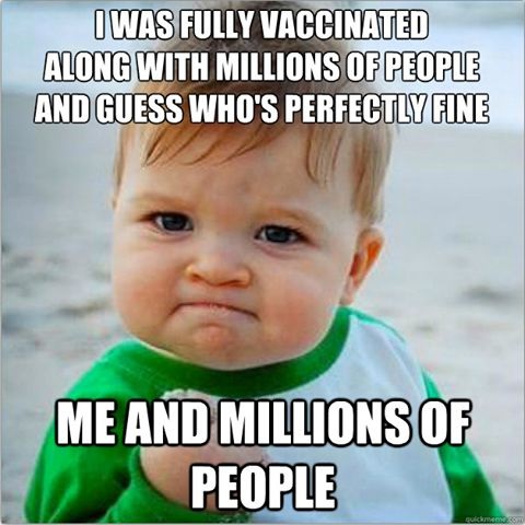
If we are going to use anecdotes, I have a few million of them for you. Image created by Melissa Miller.
Bad Argument #29). “Ian’s story.”
Bad Argument #30). “Stephanie’s story.”
Personal anecdotes are completely and totally worthless for establishing causation. Again, the fact that someone died months, weeks, or even days after a vaccination does not prove that the vaccine was the cause (i.e., these are post hoc ergo propter hoc fallacies). Further, if we are going to allow personal anecdotes, then I can easily counter stories like these with the stories of me, my three siblings, my wife, my wife’s brother, all nine of my cousins, and all of my friends, none of whom have had serious reactions to vaccines. We have to rely on carefully controlled studies, not anecdotes (details here).
Bad Argument #31). “And I couldn’t resist throwing in some celebrities who do not vaccinate their kids or at least question the effectiveness and safety of vaccines: Mayim Bialik (Amy Farah-Fowler from Big Bang Theory)”
Bad Argument #32). “Jenny McCarthy.”
Bad Argument #33). “Jim Carrey.”
Bad Argument #34). “Rob Schneider.”
Bad Argument #35). “Donald Trump.”
Bad Argument #36). “The legendary Chuck Norris.”
Bad Argument #37). “Even Dr Oz’s wife doesn’t allow him to vaccinate their kids.”
 These seven “arguments” are among the most absurd so far. The author of this article didn’t just cite a celebrity as an expert, they actually blatantly argued that you shouldn’t vaccinate because these celebrates say not to (remember the title of this article is “100 Arguments Against Vaccines”)! This is possibly the most flagrant inappropriate appeal to authority fallacy that I have ever seen (and believe me, I’ve seen a lot of appeals to authority). Who gives a crap what a bunch of celebrates think? The fact that they are famous doesn’t mean that we should we listen to their uneducated opinions. Finally, if we are going to play the celebrity card, I’m going to go with what Stephen Colbert had to say (to be clear, I’m not actually saying you should accept vaccines because Colbert does, it’s just a good quote, and it once again demonstrates that anti-vaxxers use inconsistent logic).
Bad Argument #38). “The medical profession still has no clue how the immune system really works, let alone understand the fragile immune system of a 6-week old baby! Do you really think it’s a wise idea to inject foreign DNA, heavy metals, antibiotics, GMO’s, preservatives, etc. into something if you don’t know how it works.”
That’s odd, because I could have sworn that when I took immunology a few years ago, I had to memorize exactly how the immune system works. In fact, I still have the sizable textbook from that course and it explains the immune system in excruciating detail. Not to mention the fact that literally hundreds of thousands of papers have been published about the immune system. So this claim makes no sense whatsoever. Also, it concludes with an appeal to emotion fallacy (see #10-13).
Bad Argument #39). “Vaccines are NOT ‘free,’ like the Ministry of Health, Pharmaceutical companies, doctors, etc. would have us believe. They cost the NZ tax payer millions! Oh, and we also have to pay for the damage they cause.”
The way that vaccines are paid for varies greatly from one country to the next, so whether or not this argument applies depends on the country that we are dealing with, but let’s say that it is universally true. The argument then becomes, “vaccines are bad because they cost money.” Really? We shouldn’t use something just because it costs money? Did you pay for the computer/phone that you are reading this on? Does that make it bad?
Bad Argument #40). “Pharmaceutical companies cannot be trusted! A video interview with Dr Russell Blaylock on fraudulent vaccine science and ethics – a must watch.”
Bad Argument #41). “Oh and if you need some more evidence of the untrustworthiness of pharmaceutical companies, read the book entitled ‘Diary of a Legal Drug Dealer.'”
These are just repeats of #14 so please see it. Also, Blaylock is hardly a reliable source.
Bad Argument #42). “Vaccination bypasses all the body’s natural defense systems – it’s a totally unnatural process – something we were not designed to have to deal with.”
Apparently the author doesn’t understand how vaccines work because this argument is blatantly untrue. During a “natural” infection, your immune system detects the infectious agent and instructs your body to make cells which can produce antibodies that are specific for that infectious agent. After a vaccination, your immune system detects the infectious agent in the vaccine and instructs your body to make cells which produce antibodies that are specific for that infectious agent. There is only one important difference: in the vaccine, the infectious agent has been modified or killed so that it cannot cause a full blown infection, but the way that your body responds is essentially identical. Also, note that this argument is a blatant appeal to nature fallacy. Even if the claims were true, the fact that something is unnatural does not automatically mean that it is bad.
Bad Argument #43). “Antibiotics are blamed for creating superbugs, yet they are routinely added to vaccines!”
Antibiotics themselves are wonderful. They have saved countless millions of lives. The problem is their overuse. People use them for everything, even when they aren’t really necessary. It is this overuse which causes superbugs to evolve. The superbugs are not going to spontaneously form inside the vaccine. Finally realize that the antibiotics are in there to prevent bacterial contamination. In other words, they are necessary for vaccines to be safe, and if they weren’t there, then vaccines actually would be dangerous.
Bad Argument #44). “Big Pharma keeps on increasing the amount of recommended ‘boosters’ as it’s just such a fabulous way for them to make more money without having to do any extra work.”
Actually, they are recommending boosters because the scientific evidence says that for some diseases, immunity (including natural immunity) wears off over time (Wendelboe et al. 2005). This argument is what we call a question begging fallacy. I would not accept the premise that boosters were all about money unless I had already accepted the conclusion that vaccines were bad (more details and sources on boosters and the longevity of immunity here).
Bad Argument #45). “There is no consideration for a child’s mass when they are given a vaccine – a 6 week old baby is given the same dose as a 5 year old.”
That is because vaccines have been designed to be safe the age at which they are recommended, which means that they are also safe for larger children. In other words, a dose that is designed to be safe for a 6 week old will also be safe for a 5 year old, so there is no reason to adjust the dose.
 Bad Argument #46). “Even immunologists admit that vaccines compromise our natural immunity.”
The link for this one was broken, so I don’t know which particular immunologists it was referring to, but regardless, it’s an appeal to authority fallacy. The fact that you found a few immunologists who agree with you doesn’t make you right. Also, there is scientific evidence that artificial immunity is much better than natural immunity (see #47).
Bad Argument #47). “Childhood illnesses actually help to strengthen a child’s immune system.”
They only “strengthen” the immune system in that they prevent you from getting the disease a second time. In other words, this argument boils down to, “you should get measles so that you don’t get measles” (I explained the absurdity of this in more detail here). Further, a recent study (Mina et al. 2015) found that getting a measles infection actually suppresses the immune system for 2-3 years! In other words, it weakens the immune system for up to three years after the initial infection, and during that time you are more likely to get other diseases (more details here).
Bad Argument #48). “The short term immunity that is sometimes gained from vaccination in childhood only means it is much harder for the body to deal with when that immunity has waned and you get the illness as an adult.”
I’m not sure exactly what the author is arguing here, but my guess is that they are arguing that childhood diseases are often worse if you get them as an adult, so it is better to get them as a child. If that is the case, there are several things to note. First, there are these simple, safe, and cheap things called boosters that maintain your immunity even into adulthood. Second, “natural” immunity often isn’t life long as well (details here). Finally, when most people are vaccinated, and herd immunity is high, your chance of getting an infectious disease as an adult is generally extremely low, whereas if you get the disease as a child, your chance of getting a serious complication from it is often very high. For example, for measles infections, 1 in 1,000 will die, 1 in 1,000 will get encephalitis, 1 in 20 will get pneumonia (often requiring hospitalization), and 1 in 20 will get an ear infection (sometimes resulting in permanent deafness).
Bad Argument #49). “http://www.ias.org.nz/wp-content/uploads/ias-brochure-2011.pdf.#sthash.t7LszLZf.dpuf”
This argument was simply a link, and the link is broken.
Bad Argument #50A). “Vaccines are commonly believed to work by producing antibodies. However, a number of researchers have found that the presence of antibodies only indicates that the immune system has come into contact with an antigen. What this means is that we are told of vaccines producing antibodies, which in turn will protect us against disease, is a lie! The presence of antibodies does NOT equal immunity!”
This lengthy ramble makes no sense whatsoever, and it represents a clear lack of understanding about how the immune system works. An antigen is a surface recognition protein that is present on the outer membrane of cells (or bacteria walls). Each type of cell has a specific antigen that your body can recognize (this is how your immune system tells the difference between your cells and a foreign cell). So, when you get an infection, your body learns to identify the antigens of the invading cells, and it produces antibodies for those cells. What vaccines do, is present your body with the antigens without actually giving you the infection. That way your body produces the necessary antibodies without you actually getting sick. So, the mechanism that your immune system uses is identical between vaccines and natural immunity. They both produce antibodies in response to antigens (see $42).
Bad Argument #50B). “We know what the signs and symptoms of the so called “vaccine preventable” diseases (e.g. measles, influenza, pertussis etc.) are. We know the best the treatments (natural or pharmaceutical) for each. However, once vaccinated, possible side effects from the vaccinations (all noted in the insert leaflets) are many and various, and may or may not be successfully dealt with.”
First, this argument ignores that fact that despite our medical knowledge, these diseases often have serious consequences, including death (see #48). Second, we know what the side effects of vaccines are, and serious side effects are extremely rare. For example, for the MMR vaccine, the most common serious side effect is an allergic response, but it only occurs in about 1 in every 1,000,000 cases. Further, it’s going to occur right after the injection, which means that it will happen at a medical facility where treatment is readily available. Finally, the vaccine inserts list every condition that has ever been reported following a vaccine, but that does not mean that the vaccine caused those conditions (that’s a post hoc ergo proter hoc fallacy). You can find a more detailed explanation of the vaccine inserts here.
Bad Argument #51). “This ’60 Minutes’ program was on in July 2011 and looks at two New Zealand children who were brain damaged by the whooping cough vaccine and another who was killed by the Gardasil vaccine. During June 2005 and June 2011, ACC paid out on 449 claims of vaccine damage.”
First, remember again that the fact that an injury follows a vaccine doesn’t automatically mean that the vaccine caused it (this is yet another post hoc ergo proter hoc fallacy). Second, let’s assume that the vaccine was actually responsible. If that’s the case, the vaccine is still the safer option. Vaccines have side effects, no one has ever denied that, but they are safer than the alternative, and two cases of brain damage aren’t nearly as troubling as the numerous deaths that occur without the vaccine. Whooping cough still kills thousands of people annually. In 2008 alone, it killed 195,000 children, and during that same year, the vaccine was estimated to have saved 687,000 lives. So please, stop trying to scare me with your cherry-picked examples. Finally, regarding the claims of vaccine damage, it’s a no fault system and does not constitute evidence that the vaccine actually caused the problem (see #26).
Bad Argument #52). “The Hippocratic Oath states that physicians swear to do no harm – yet vaccines routinely destroy the lives of people right around the world.”
No they freaking don’t! They do, however, dramatically reduce disease and death rates (Clemens et al. 1988; Adgebola et al. 2005; Richardson et al. 2010).
Bad Argument #53). “The polio vaccine actually causes vaccine induced polio paralysis.”
The link for this one goes to a Natural News article, not a legitimate source, and it claims that vaccines are causing non-polio acute flaccid paralysis (NPAFV). This claim is not supported by scientific evidence. It is true that the rates of NPAFV have increased in some areas, but they are caused by various bacteria and viruses, not vaccines (Laxmivandana et al. 2013). Also, to be fair, in extraordinarily rare cases in populations with very low vaccination rates, the virus in the vaccine can mutate to a form that causes polio and can cause paralysis (details here). There have, however, only been a total of 758 cases of this despite millions of vaccinations. Further, let’s not forget that the vaccine has completely eliminated polio from many countries. So overall, the paralysis rates are much, much lower with the vaccine than without it.
Bad Argument #54). “Vaccines accomplishing world depopulation.”
Oh for goodness sake. This claim links to a video where Bill Gates is talking about slowing the human population growth rate and says that vaccines are very useful in accomplishing that; however, slowing the growth rate and depopulating are two entirely different things. As countries get access to technology and proper medical care, people start having fewer children because they don’t need to have as many, since most of them actually survive into adult hood. Vaccines slow the growth rate because when all your children survive, you only need to have one or two; whereas when most of them die in infancy, you need to have a lot. This is a well established fact: in developed countries, people choose to have fewer children. That is completely and totally different from vaccines causing sterility, deaths, etc. Only in the mind of a paranoid conspiracy theorist could Gates’ comment ever be twisted into something sinister.
Bad Argument #55). “GlaxoSmithKline were responsible for the death of 14 babies during illegal vaccine experiments.”
This is a gross misrepresentation. First, the experiment itself was not illegal, but it appears that proper consent was not obtained for all subjects. Importantly, however, the 14 deaths were not associated with the vaccine being tested, because those 14 children were given the placebo! The very article that the author(s) cited says this. So the claim that GlacoSmithKline was responsible for these deaths is an outright lie.
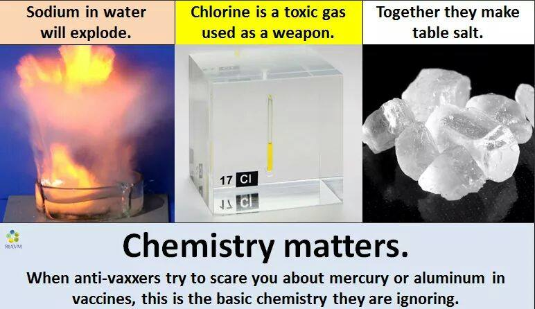
Image via Refutations to Anti-Vaccines Memes
Bad Argument #56). “Even though mercury has been linked to numerous illnesses, it is still routinely used in vaccines.”
First, the mercury in vaccines is ethyl mercury, whereas the toxic mercury is methyl mercury. They are completely different. Further, ever since 2001, ethyl mercury has only been included in some forms of the flu vaccine. Also, the dose makes the poison, and the amount in vaccines is tiny (more details here and here).
Bad Argument #57). “Fully vaccinated doctors get whooping cough – so what’s the point in getting vaccinated.”
Just because something isn’t 100% effective doesn’t mean that it isn’t worth using (see #2). This argument is like saying, “even the people who design air bags have fatal car accidents, so what’s the point of having airbags?”
Bad Argument #58). “Vaccine ingredients can lead to a severe form of kidney disease.”
The dose makes the poison, and the dose in vaccines is tiny. The fact that an ingredient can be harmful in a high dose does not mean that it is harmful in a low dose.
Bad Argument #59). “The whole policy of vaccination is based on money, not on health, safety or anything else that might benefit the human race.”
Actually, pharmaceutical companies make very little from vaccines (details here), and there are many independent scientists and doctors involved (more details here). Further, even if money was the sole goal, that wouldn’t constitute evidence that vaccines aren’t safe and effective. If we were to apply this line of reasoning consistently, then since the whole point of Toyota is to make money, Toyotas must be dangerous.
Bad Argument #60). “Vaccines are the cause for many of the chronic diseases we see these days.”
No they aren’t. Their safety has been rigorously tested over and over again. You cannot make this claim unless you can back it up with properly controlled studies with large sample sizes that were published in reputable peer-reviewed journals. The anecdotes in the link that the author(s) cite just doesn’t cut it.
Bad Argument #61). “Vaccines are used to commit genocide among First Nations people in Canada.”
The “source” for this claim is a “Wholistic Nutrition Counsellor” who was unhappy that Xyolhemeylh Health and Family Services supported vaccines rather than her definition of healthy living, which is, “learning about the connection between body, mind and spirit and allowing the body to heal itself using whole foods, organics, natural medicines.” In other words, she was disgruntled about being asked to recommend science instead of woo. She provides absolutely zero evidence of genocide. The closest that she comes is saying, “I had observed a high incedence [sic] of deaths within the Sto:Lo communities linked to suicides, diabetes, cancer, heart disease,” but I seriously doubt that vaccines cause suicides. So, instead of providing actual evidence of genocide, she simply states that vaccines were being pushed, then gives the usual nonsense arguments about “dangerous toxins” and side effects. In other words, this argument is a question begging fallacy. I wouldn’t believe that the vaccines were being used for genocide unless I was already convinced that the vaccines were dangerous. Finally, one of her cornerstone arguments is that she was instructed not to talk to families about the risks of vaccines. She presents this as evidence of a conspiracy, but that request actually seems completely reasonable given that she would almost certainly have given the families misinformation about “toxins” and encouraged people to rely on diet and exercise rather than vaccines.
Bad Argument #62). “Vaccination is not compulsory in New Zealand or the United States – we have the right to refuse to undergo medical treatment.”
I also have the right to eat nothing but lard until I become Jabba the Hutt, but that doesn’t mean that it’s a good idea. The simple fact that you have the right to do something is not a valid argument for actually doing that thing.
Bad Argument #63). “If you’re religious, then there are plenty of reasons to not vaccinate.”
It would take an entire post to explain the many problems in the various religious arguments, so I will just summarize by saying that if your religion actually says that you should let your children suffer and die rather than using a simple preventative measure, then there is something seriously wrong with your religion. Also, relying on God to protect your child seems rather foolish given the thousands of deaths that occurred prior to vaccines (why didn’t God save those children?).
Bad Argument #64). “More information is becoming available regarding the link to vaccines and Sudden Infant Death Syndrome (SIDS).”
As usual, the link for this claim goes to an anti-vaccine page rather than a legitimate source, and the anti-vaccine page contains various anecdotes, post hoc ergo propter hoc fallacies, correlation fallacies, and shoddy preliminary studies. In contrast, multiple peer-reviewed studies have found that not only do vaccines not increase the risk of SIDS, but is some cases, they may actually lower the risk (Hoffman et al. 1987; Griffin et al. 1988; Mitchell et al. 1995; Fleming et al. 2001; Vennemann et al. 2007a; Vennemann et al. 2007b).
Bad Argument #65). “Most doctors have no idea what ingredients are found in vaccines. If you don’t believe me, ask your doctor at your next visit! Why would you allow your doctor to inject you with something when they do not even know its ingredients?”
Most mechanics don’t know the chemical ingredients in engine oil, so why would you allow them to fill your engine with something when they don’t even know its ingredients? Hopefully you see my point. You don’t have to know every single ingredient to know that something is safe and effective (again, anti-vaccers suck at consistent reasoning). I don’t care if my doctors know the chemical makeup of a vaccine or pharmaceutical, just so long as they know the literature and know the risks and benefits associated with a vaccine/treatment (which they do, btw).
Bad Argument #66). “Only about 1% of serious events are reported to the FDA. That means that 99% of adverse vaccine reactions are not reported.”
First, realize that the 1% number was cherry-picked, and both the opinion paper that the author cited (Kessler 1993) and the study that generated the 1% number (Scott et al. 1987) are rather old and almost certainly don’t reflect the current values. Indeed, a slightly more recent systematic review found that on average 20% of serious events were reported (Hazell and Shakir 2006). Further, those values are for adverse reactions to any drug. You cannot apply a broad generality to something as specific vaccines. Indeed, it seems that the reporting rates for vaccines are much higher (Hazell and Shakir 2006). In fact, vaccine injuries are often over-reported, because many of the cases that get reported to the VAERS are false associations (i.e., an injury followed the vaccine, but the vaccine didn’t actually cause it; see #26).
Bad Argument #67). “The pertussis (whooping cough) bacteria are adapting to the vaccine and mutating, much like antibiotic resistant superbugs, becoming more pronounced.”
First, there is very little scientific evidence to support this argument (Cherry 2012), and the scientific studies that anti-vaccers cite to bolster this claim are always terribly misconstrued. Nevertheless, for sake of argument, let’s assume that pertussis is evolving to “resit” the vaccine. If that were true, the solution would simply be to modify the vaccine. This situation is totally different from antibiotics. You see, antibiotics actually kill bacteria, and the bacteria evolve so that the antibiotics no longer kill them. In contrast, vaccines don’t kill bacteria, viruses, etc. Rather, they teach the immune system how to recognize them. So the only way to mutate such that a vaccine no longer works, would be to mutate a different antigen (surface recognition protein). In other words, if the vaccine teaches the immune system to look out for antigen X, but a bacteria has mutated so that it now has antigen X’, the vaccine will no longer work. Fixing this is, however, extremely simple: just modify the vaccine so that it contains both antigen X and X’.
Bad Argument #68). “30 Years of secret official transcripts show UK Government experts cover up vaccine hazards to sell more vaccines and harm your kids.”
This claim is based on the following report, which claims to have documented 30 years of admittedly disturbing corruption among UK officials. Wading through all of the documents that the report cites would take me days, so instead, let’s just assume that the original report is correct. Even if it is, the claims made by the anti-vaccers are outrageous and unmerited. I see anti-vaccers all over the internet claiming that this report proves that the officials knew that vaccines were dangerous, knew that they didn’t work, tried to stop safety studies, etc. Similarly, the Natural Health Warrior article claims that the officials were trying to “harm your kids.” The reality is that the report simply claimed that officials tried to downplay the side effects of vaccines and prevent parents from knowing about them. There is nothing in the report to indicate that they knew that vaccines didn’t work, were trying to harm children, etc. In fact, the opposite is true. The report says, ”
“Here I present the documentation which appears to show that the JCVI made continuous efforts to withhold critical data on severe adverse reactions and contraindications to vaccinations to both parents and health practitioners in order to reach overall vaccination rates which they deemed were necessary for ‘herd immunity.'”
In other words, the officials were withholding information because they knew that vaccines worked and wanted to make sure that the vaccination rate was high enough to protect everyone. To be clear, people do have the right to know about the side effects of vaccines (even if they are rare and minor, see #1 and 3), but the evidence in the report in no way shape or form justifies that claims being made by anti-vaccers, and it most certainly doesn’t demonstrate or even suggest that vaccines are ineffective or dangerous.
Bad Argument #69). “If you need any further evidence regarding the numerous errors that occur during vaccine manufacturing, storing, administering, etc. then here is a great resource.”
The link for this specific “resource” is broken, but it was something from vaccinetruth.org, which is one of the most counterfactual websites in existence. There is nothing on that website that constitutes a “great resource.” Please see #18 for information on how absurdly tightly regulated the manufacturing process actually is.
Bad Argument #70). “The head of the Center for Disease Control – Julie Gerberding – admits in this interview that vaccines can cause autism-like symptoms. Same difference!”
First, that’s not exactly true. She admitted that vaccines can cause fevers (which we already knew), and in certain cases where a person has other conditions that are already stressing the body (specifically rare mitochondrial disorders), that fever can trigger changes that result in autism-like symptoms. That is extremely different from a broad generalization that “vaccines can cause autism-like symptoms.” Further, the specific case in question is that of Hannah Poling, and it is not at all clear that vaccines were at fault (Doja 2008; Offit 2008; see #15 for more on vaccines and autism).
Second, autism and autism-like symptoms are not in anyway the same thing. Rhinovirus (one of the causes of the common cold) produce hay fever-like symptoms, but that does not mean that Rhinoviruses cause hay fever. This argument commits a logical fallacy known as affirming the consequent.
Note: the “source” for this claim is a Natural News video (“CDC Chief Admits That Vaccines Cause Autism”) that chopped and misrepresented an interview with Gerberding. The key statement occurs at 2:50.

Correlation does not equal causation. Organic food sales and autism rates are tightly correlated, but that does not mean that organic food causes autism. Image via the Genetic Literacy Project
Bad Argument #71). “Vaccines are the cause for the alarming rise in peanut allergies around the world. When I was a child, I didn’t know a single kid with a peanut allergy in our entire school. These days, peanut-containing products are banned from most school grounds to prevent deadly anaphylactic shock in those who are allergic to peanuts.”
There is no scientific evidence to support the claim that vaccines or their ingredients cause peanut allergies. The fact that vaccines have increased along with the increase in peanut allergies does not mean that vaccines cause peanut allergies. This is a correlation fallacy.
Bad Argument #72). “Yeast is a common ingredient in vaccine manufacturing and has been linked to the rise and cause of asthma in many young children.”
Asthma rates are actually lower among vaccinated children than unvaccinated children (Grabenhenrich et al. 2014).
Bad Argument #73). “Vaccines cause allergies because they clog our lymphatic system and lymph nodes with large protein molecules which have not been adequately broken down by our digestive processes, since vaccines by pass digestion with injections.”
Essentially nothing about this claim is true. Vaccines don’t “clog” our lymphatic system (remember, proteins are microscopic), and although some people are naturally allergic to the ingredients in vaccines, there is no evidence that vaccines cause allergies.
Bad Argument #74). “There was a 4,250% increase in fetal deaths reported to VAERS after the flu vaccine was given to pregnant women.”
First, remember that VAERS is completely self reported and the fact that someone reported a fetal death following a vaccine does not mean that the vaccine was responsible (more details here and here). Therefore, this argument is totally invalid. Second, and more importantly, numerous peer-reviewed studies have examined the effects of flu vaccines on fetal moralities and, guess what, they have all found that flu vaccines do not increase the risk of fetal deaths (Mak et al. 2008; Pasternak et al. 2012a; Fell et al. 2012; Haberg et al. 2013). Similarly, studies have also failed to find increased risks to infants whose mothers were vaccinated during pregnancy (Fell et al. 2012; Pasternak et al. 2012b). You can also find a refutation of the study that produced the 4,250% figure here.
Bad Argument #75). “AIDS was transmitted to the human race via the monkey cells used to make vaccines. I challenge you to listen to this interview with Merck vaccine scientist Dr Maurice Hilleman who admits “I didn’t know we were importing the AIDS virus at the time.”
The claim that the polio vaccine spread AIDs has been thoroughly refuted by scientific tests (Sharp, et al. 2001), including directly testing the vaccine for the presence of HIV (Berry, et al. 2001; Blancou, et al. 2001) and looking at the phylogenetics of the virus and its wild hosts (Rambaut, et al. 2001; Worobey, et al. 2004). You can find more complete summaries of the science here and by Weiss (2001). You can also find an explanation of the actual interview at Respectful Insolence.
Bad Argument #76). “Disease outbreaks still occur in fully and highly vaccinated communities.”
True, but they are often triggered by an unvaccinated person, they are usually easily contained, and they are less common than outbreaks in communities with low vaccine levels. Ultimately, this argument is a sharpshooter fallacy because it ignores the fact that overall, disease rates are much lower among the vaccinated (important sources in #8 and more details here).
Bad Argument #77). “Newly vaccinated individuals are responsible for the spread of disease via ‘shedding’ from live virus vaccines.”
It is important realize that they are “shedding” the inactivated virus that is used in the vaccine. In other words, you cannot get the full disease itself from the shed virus. All you can get is the modified version of the virus that is used in the vaccine. So for most people, this is not a problem, but it can be a problem for people who are immunocompromised, which is why they are encouraged to avoid the feces of those who have been recently vaccinated (which they probably should be doing anyway). To quote the very study that the Natural Health Warriors post cited (Anderson 2008), “Since the risk of vaccine transmission and subsequent vaccine-derived disease with the current vaccines is much less than the risk of wildtype rotavirus disease in immunocompromised contacts, vaccination should be encouraged” (my emphasis).
Bad Argument #78). “Pro-vaccination enthusiasts like to point to pharmaceutical industry sponsored research for evidence that vaccines work. In this interesting article by John Ioannidis, he writes why most published research findings are false.”
This argument is a gross misrepresentation of Ioannidis’s informative work. The main problem that Ioannidis was dealing with was the fact that statistics inevitably produce some false positives, and there is a strong publication bias towards positive results. Thus, many initial studies get published because they got a positive result, but they are later refuted when other studies can’t replicate the results. In other words, this is a problem that mostly arises when there is only one or two papers on a topic. It does not apply to situations like vaccines where you have literally thousands of papers that all agree with each other. Where it does apply, however, is the occasional peer-reviewed anti-vaccine paper that disagrees with all of the other vaccine research. The take home message from Ioannidis is not that we shouldn’t trust science, but that we should critically evaluate papers and look at the literature as a whole rather than focusing on a single study (more details here and here). Finally, many of the studies on vaccines were not sponsored by pharmaceutical companies (details here).
Bad Argument #79). “Those who promote vaccines also happen to be the ones who benefit from it financially”
That is often untrue (details here). Also, let’s not forget that many of the people who oppose vaccines benefit from doing so. For example, Natural News (which the Natural Health Warriors post cites religiously) has a store where they sell you their alternatives to vaccines, so this is a clear case of inconsistent reasoning (details here).
Bad Argument #80). “Some doctors in New Zealand are either intentionally lying about the effectiveness of vaccines, or they are just incredibly ignorant. One such example is Dr John Cameron, who blatantly lied (with a smile on his face) about the flu vaccine on “Campbell Live” earlier this year, and here is the IAS’s response.”
The link to IAS’s response is broken, so I don’t know exactly which claims are being referred to as lies, but the vast majority of the doctor’s claims in the video are backed by solid scientific evidence. The only claims that were suspect were the claim that the flu leads to suicides (I have no idea if that claim is correct or not) and the claim that you can’t even get a mild fever from the flu vaccine (I’m pretty sure that this claim is in fact incorrect); however, neither of those potential errors match the accusation, and even if they did, so what!? Just because one doctor is ignorant doesn’t mean that the flu vaccine doesn’t work (that’s a guilt by association fallacy).
Bad Argument #81). “Courtesy of Dr Goldman: Prior to the universal varicella vaccination program, 95% of adults experienced natural chickenpox (usually as school aged children) These cases were usually benign and resulted in long term immunity. This high percentage of individuals having long term immunity has been compromised by mass vaccination of children which provides at best 70 to 90% immunity that is temporary and of unknown duration, shifting chickenpox to a more vulnerable adult population where chickenpox carries 20 times more risk of death and 15 times more risk of hospitalization compared to children.”
See #48. Also, the overall rates of deaths from chicken pox have dropped markedly following the introduction of the vaccine (Nguyen et al. 2005).
Bad Argument #82). “Many parents have commented that their unvaccinated children are much healthier than their vaccinated children. Here is a blog to read on one such mum’s journey.”
Anecdotes are meaningless. The scientific data show that vaccinated children are healthier (Schmitz et al. 2011). See #7, 29, and 30.
Bad Argument #83). “Why bother getting the flu shot? At best, vaccines are effective against only influenza A and B, which represent only about 10% of all circulating viruses. Therefore, there is a 90% chance you will not even be exposed to an influenza virus.”
How about the fact that during the 1989-1990 outbreak, those who were vaccinated had a 41% lower mortality rate than the unvaccinated (Ahmed et al. 1995)? Influenza is complicated because it constantly evolves. As a result, flu vaccines are not always as effective as most other vaccines, and there is certainly room for improvement, but your odds of getting the flu are generally lower with the vaccine (Osterholm et al. 2012). Also, although not identified in Osterholm’s review, other studies have found that the vaccine is particularly important for the elderly (Nordin et al. 2001).
Bad Argument #84). “Here is a great resource showing cases that were awarded damages by the US Government via the Vaccine Court, which is a federal court of claims for the flu vaccine. Note the number of deaths, in just 2012.”
See #26. Court rulings do not constitute evidence that vaccines are dangerous (judges aren’t doctors or scientists).
Bad Argument #85). “If you’re not yet aware of the lies and scare mongering surrounding the 2006 Bird Flu saga, then start your journey here.”
Seventy-nine deaths across nine countries certainly sounds like cause for concern to me. More importantly, we didn’t have a vaccine for the bird flu in 2006, and even now we are still in the trial stages, so how exactly is this argument about vaccines?
Bad Argument #86). “Oh and don’t forget the Swine Flu hype! History is always repeating itself, so be prepared for more Big Pharma induced scare mongering in the future – with matching vaccines to “save us all” of course!”
Each year in the US alone influenza causes anywhere from 3,300 to 48,600 deaths annually (CDC 2010)! That’s not fear-mongering, that’s a simple fact. The callousness of the anti-vaccine movement astounds me.
Bad Argument #87). “Hassle the Ozzies all you like, but at least they are waking up to the dangers of vaccination, with a 600% increase in the number of parents refusing to vaccinate.”
This is an appeal to popularity fallacy.
Bad Argument #88). “Gardasil contains polysorbate 80, also known as Tween 80, which has been linked to infertility in mice.”
The dose makes the poison. See #10-13.
Bad Argument #89). “An eye-opening report from the International Medical Council on Vaccination.”
Despite its scientific sounding name, the IMCV is a quack group devoted to anti-vaccine ideology. So it’s not a legitimate source. Also, the report in question is full of the typical anti-vaccine drivel that I have spent this entire post refuting.
 Bad Argument #90). “More deaths following the MMR vaccine.”
This is yet another post hoc ergo propter hoc fallacy. The fact that an infant died shortly after receiving a vaccine does not mean that the vaccine was responsible. See #23, 24, 29, 30 and 50B.
Bad Argument #91). “This brave Queensland Police officer speaks out about vaccine damaged children being written off as cases of Sudden Infant Death Syndrome (SIDS). If only we had more people brave enough to come out and speak the truth about vaccines.”
This isn’t actually an argument, so there is nothing for me to say here (except of course that in some cases vaccines may actually reduce the risk of SIDS [see sources in #64]).
Bad Argument #92). “A University of Pittsburgh study showed that monkeys developed autism-like reactions when given the same vaccines as children.”
That study (Hewitson et al. 2010) was a preliminary pilot study (the term “pilot study” was literally in its title). The full study with a complete sample size just came out and, as often is the case in science, the preliminary results were wrong. There were no differences between vaccinated and unvaccinated monkeys (Gadad et al. 2015; more details here).
Bad Argument #93). “It’s all about the money, honey.”
No, it’s not, and even if it was, that wouldn’t mean that vaccines don’t work/aren’t safe. See #6, 14, and 59.
Bad Argument #94). “If you’d like some real-life stories of vaccine reactions, you’ll find them on this Facebook page.”
Good grief, how many times do I have to say this: anecdotes are meaningless; only peer-reviewed studies matter! See #7, 29, 30, and 82.
Bad Argument #95). “Serious neurologic, thromboembolic, and autoimmune complications have been reported in patients who received human papillomavirus (HPV) vaccines.”
First, vaccines do admittedly have side effects but serious complications are rare (see #2 and 3). In this case, however, a large cohort study failed to find evidence that the HPV vaccine causes serious neurological, thromboembolic, or autoimmune complications (Arnheim-Dahlstrom et al. 2013).
Bad Argument #96). “And if you’d like just a little more evidence of the fraudulent activities of Big Pharma, have a read of this.”
Once again, I trust the science not the companies who benefit from it. See #14.
Bad Argument #97). “Dr Janet tells us the real reasons behind why doctors push vaccines.”
Perhaps it’s because they actually care about their patients, and (unlike anti-vaccers) they are scientifically literate and realize that literally thousands of studies have shown that vaccines are safe and effective…literally thousands!
Bad Argument #98). “This resource lists some great books about vaccination, with plenty of reasons to not vaccinate.”
Again, the scientific evidence clearly shows that vaccines are safe and effective. Books, blogs, and anecdotes are irrelevant. Until you can back up your position with peer-reviewed literature, you don’t have an argument.
Bad Argument #99). “Information on the link between diabetes and vaccination.”
What a surprise, they cited more anecdotes and post hoc ergo propter hoc fallacies. Unsurprisingly, the actual studies have found that vaccines do not increase the risk of developing diabetes (Jefferson and Demicheli. 1998; DeStefano et al. 2001).
Bad Argument #100). “And argument number 100 to NOT vaccinate: listen to your gut instinct.”
 This argument beautifully sums up the entire anti-vaccine movement. It is a bold statement that boils down to, “screw the facts, I know I’m right and you’ll never convince me otherwise.” The anti-vaccine movement has absolutely nothing to do with facts, evidence, or legitimate concerns. It is all about fear, assumptions, a herd mentality, and “mommy instincts.” As should be very clear by this point, the scientific evidence is overwhelmingly on the side of vaccines. All throughout this post, I have cited study after study that has shown that vaccines are safe and effective, but those studies don’t matter to anti-vaccers. They have decided that vaccines are dangerous and no amount of evidence will ever convince them otherwise. This is why their position is so laughably absurd.
P.S. my gut tells me that if you honestly think that your gut is a more reliable source of scientific information than thousands of peer-reviewed studies, then you’re an idiot. I generally try very hard to avoid calling people “idiots” on this blog (believe me it is really hard sometimes), but in this case there is no other way to accurately describe the situation. Trusting your gut instead of scientific evidence is an inexcusable level of willful ignorance that can only be described as stupidity. It’s one thing to be uniformed but willing to learn. It is something else entirely to refuse to listen to contrary evidence and insist that you are right even though you are clearly wrong.
Note: All links to scientifically inaccurate websites are redirected through donotlink.com to avoid boosting those websites’ ratings.
Note: I have made several updates to this article to include additional sources (or in some cases clarifications) that were recommended by readers. Many thanks to everyone who has made these suggestions.
Peer-reviewed sources
I apologize that some of these are behind paywalls. You may be able to get copies through your library or by simply emailing the authors.
- Adegbola et al. 2005. Elimination of Haemophilus influenzae type b (Hib) disease from The Gambia after the introduction of routine immunisation with a Hib conjugate vaccine: a prospective study. Lancet 366:144–150.
- Ahmed et al. 1995. Reduction in mortality associated with influenza vaccine during the 1989–90 epidemic. Lancet 346:591–595.
- Anderson. 2008. Rotovirus vaccines: viral shedding and risk of transmission. Lancet Infectious Disease 8:642–649.
- Anjali et al. 2015. Autism occurrence by MMR vaccine status among US children with older siblings with and without autism. Journal of the American Medical Association 313: 1534–1540.
- Antona et al. 2013. Measles elimination efforts and 2008–2011 outbreak, France. Emerging Infectious Diseases 19:357.
- Arnheim-Dahlstrom et al. 2013. Autoimmune, neurological, and venous thromboembolic adverse events after immunisation of adolescent girls with quadrivalent human papillomavirus vaccine in Denmark and Sweden: cohort study. BMJ 347:f5906
- Berry, et al. 2001. Vaccine safety: analysis of oral polio vaccine CHAT stocks. Nature 410:1046–1047.
- Blancou, et al. 2001. Polio vaccine samples not linked to AIDs. Nature 410:1045–1046.
- Cherry. 2012. Epidemic pertussis in 2012—The resurgence of vaccine preventable disease. 367:785–787.
- DeStefano et al. 2001. Childhood vaccinations, vaccination timing, and risk of type 1 diabetes mellitus. Pediatrics 108:e112.
- Doja. 2008. Genetics and the myth of vaccine encephalopathy. Paediatrics and Child Health 13:597–599.
- Fell et al. 2012. H1N1 influenza vaccination during pregnancy and fetal and neonatal outcomes. American Journal of Public Health 102:e33–e40.
- Ferris et al. 2014. Long-term study of quadrivalent human papillomavirus vaccine. Pediatrics 134: e657-665.
- Fleming et al. 2001. The UK accelerated immunization programme and sudden unexpected death in infancy: case-control study. BMJ 322:822.
- Gadad et al. 2015. Administration of thimerosal-containing vaccines to infant rhesus macaques does not result in autism-like behavior or neuropathology. Proceedings of the National Academy of Science 112:12498–12503.
- Gangarosa et al. 1998. Impact of anti-vaccine movements on pertussis control: the untold story. Lancet 351:356–391.
- Grabenhenrich et al. 2014. Early-life determinants of asthma from birth to age 20 years: a German birth cohort study. Journal of Allergy and Clinical Immunology 133:979–988.
- Griffin et al. 1988. Risk of sudden infant death syndrome after immunization with the Diphtheria–Tetanus–Pertussis vaccine. New England Journal of Medicine 319:618–623.
- Haberg et al. 2013. Risk of fetal death after pandemic influenza infection or vaccination during pregnancy. New England Journal of Medicine 368:33–340.
- Hahne et al. 2009. Rubella outbreak in the Netherlands, 2004-2005: high burden of congenital high burden of congenital infection and spread to Canada. Pediatric Infectious Disease Journal 28:795–800.
- Hammarlund et al. 2003. Duration of antiviral immunity after smallpox vaccination. Nature Medicine 9:1131–1137.
- Hazell and Shakir. 2006. Under-reporting of adverse drug reactions: a systematic review. Drug Safety 29:385–396.
- Hewitson et al. 2010. Influence of pediatric vaccines on amygdala growth and opoid ligand binding in rhesus macaque infants: a pilot study. Acta Neurobiological Experimentals 70:147–164.
- Hoffman et al. 1987. Diphtheria-Tetanus-Pertussis immunization and sudden infant death: results of the national institute of child health and human development cooperative epidemiological study of sudden infant death syndrome risk factors. Pediatrics 79:598–611.
- Hurwitz et al. 2000. Effectiveness of influenza vaccination of day care children in reducing influenza-related morbidity among household contacts. 284: 1677–1682.
- Idbal et al. 2013. Number of antigens in early childhood vaccines and neurophsychological outcomes at age 7–10 years. Pharmacoepidemiology and Drug Safety 22:1263–1270.
- Ioannidis. 2005. Why most published research findings are false. PLoS Medicine 2:e124.
- Jain et al. 2015. Autism occurrence by MMR vaccine status among US children with older siblings with and without autism. Journal of the American Medical Association 313:1534–1540.
- Jefferson and Demicheli. 1998. No evidence that vaccines cause insulin dependent diabetes mellitus. Journal of Epidemiology and Community Health 52:674–675.
- Jokinen et al. 2007. Cellular immunity to mumps virus in young adults 21 years after measles-mumps-rubella vaccination. Journal of Infectious Diseases 196:861–867.
- Kessler. 1999. Introducing MEDWatch: a new approach to reporting medication and device adverse effects and product problems. Journal of the American Medical Association 269:2765–2768.
- Knol et al. 2013. Large ongoing measles outbreak in a religious community in the Netherlands since May 2013. Eurosurveillance 18: pii-20580.
- Kramarz et al. 2000. Does influenza vaccination exacerbate asthma?: Analysis of a large cohort of children with asthma. Archives of Family Medicine 9:617-623.
- Laxmivandana et al. 2013. Characterization of the non-polio enterovirus infections associated with accurate flaccid paralysis in south-western India. PLoS ONE 8:e61650.
- Mak et al. 2008. Influenza vaccination in pregnancy: current evidence and selected national policies. Lancet Infectious Diseases 8:44–52.
- Mina et al. 2015. Long-term measles-induced immunomodulation increases overall childhood infectious disease mortality. Science 348:694–699.
- Mitchell et al. 1995. Immunisation and the sudden infant death syndrome. Archives of Disease in Childhood 73:498–501.
- Monto et al. 1970. Modification of an outbreak of influenza in Tecumseh, Michigan by vaccination of schoolchildren. Journal of Infectious Diseases 122:16–25.
- Nguyen et al. 2005. Decline in mortality due to Varicella after implementation of Varicella vaccination in the United States. New England Journal of Medicine 352:450–458.
- Nordin et al. 2001. Influenza vaccine effectiveness in preventing hospitalizations and deaths in persons 65 years or older in Minnesota, New York, and Oregon: Data from 3 health plans. Journal of Infectious Diseases 184:665–670.
- Osterholm et al. 2012. Efficacy and effectiveness of influenza vaccines: a systematic review and meta-analysis. Lancet Infectious Diseases 12:36–44.
- Pasternak et al. 2012a. Vaccination against pandemic A/H1N1 2009 influenza in pregnancy and risk of fetal death: cohort study in Denmark. BJM 344:e2794.
- Pasternak et al. 2012b. Risk of adverse fetal outcomes following administration of a pandemic influenza A(H1N1) vaccines during pregnancy. Journal of the American Medical Association 308:165–174.
- Rambaut, et al. 2001. Human immunodeficiency virus: phylogeny and the origin of HIV-1. Nature 410:1047–1048.
- Ramsay et al. 2003. Herd immunity from meningococcal serogroup C conjugate vaccination in England: database analysis. BMJ 7385: 365–366.
- Reichert et al. 2001. The Japanese experience with vaccinating schoolchildren against influenza. New England Journal of Medicine 344: 889–896.
- Richardson et al. 2010. Effect of Rotovirus vaccination on death from childhood diarrhea in Mexico. New England Journal of Medicine 362:299–305.
- Rudenko, et al. 1993. Efficacy of live attenuated and inactivated influenza vaccines in schoolchildren and their unvaccinated contacts in Novgorod, Russia. Journal of Infectious Diseases 168: 881–887.
- Sharp, et al. 2001. The origins of acquired immune deficiency syndrome viruses: where and when? Philosophical Transactions of the Royal Society of London B 356:867–876.
- Schmitz et al. 2011. Vaccination status and health in children and adolescents. Medicine 108:99–104.
- Scott and Rosenbaum. 1987. Rhode Island physicians’ recognition and reporting of adverse drug reactions. Rhode Island Medical Journal 70:311–316.
- Taylor et al. 2014. Vaccines are not associated with autism: an evidence-based meta-analysis of case-control and cohort studies. Vaccine 32: 3623–3629.
- Vennemann et al. 2007a. Sudden infant death syndrome: No increased risk after immunisation. Vaccine 25:336–340.
- Vennemann et al. 2007a. Do immunisations reduce the risk of SIDS? A meta-analysis. Vaccine 26:4875–4879.
- Vincenzo et al. 2014. Long-term efficacy and safety of human papillomavirus vaccination. International Journal of Women’s Health 6:999–1010.
- Weiss. 2001. Polio vaccines exonerated. Nature 410:1035:1036
- Wendelboe et al. 2005. Duration of immunity against pertussis after natural infection or vaccination. Pediatric Infectious Disease Journal 24:S58–S61.
- Worobey, et al. 2004. Origin of AIDS: contaminated polio vaccine theory refuted. Nature 428:820–820.